Quickstart guide
Select from the topics below to get a quick overview of
where to find options and how to set up a first model. For detailed information
on each page of the GUI, please see information on GUI
components.
Quick overview of the GUI
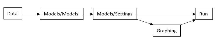
The program utilizes six pages to set up and perform an HLM
or GLIM analysis. These appear in order at the top of the page in the sequence
they would be used to set up a new analysis: MLC, Data, Models
(including Settings), Graphing and Run. The diagram below
shows the general order of operations:
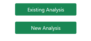
 The Welcome or landing page that opens when first
starting the program offers the user two options. One can either read in
information on a previous analysis by clicking the Old Analysis option,
or start with a new analysis using the New Analysis option.
The Welcome or landing page that opens when first
starting the program offers the user two options. One can either read in
information on a previous analysis by clicking the Old Analysis option,
or start with a new analysis using the New Analysis option.
-
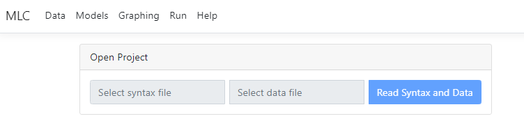
If Existing Analysis is
clicked, the user is prompted for the name of the previously save MLCJSN file
that contains the model specifications and the name of the data file used for
the model. Once supplied, all the other pages will be populated with the
information from the MLCJSN file and the model can be rerun or adapted as
needed prior to running amended syntax. By default, the program will
automatically take the user to the Models page.
-
If New Analysis is
clicked, the Data page will open. The Data page is used to read
in data. Currently, only CSV (comma separated values) files can be used as
input. Data may be read in from the user’s local hard drive disk, One
Drive or Google Drive.
 The Models page is used to specify the model to be
fitted. It consists of two parts, Models and Settings.
On the Models page, the model to be fitted is set up (for a new analysis) or displayed (for an old
analysis) as a set of level-1, level-2, and level-3 equations. The Models
page must be completed after completion of the Data page, but before the
Settings page is accessed.
The Models page is used to specify the model to be
fitted. It consists of two parts, Models and Settings.
On the Models page, the model to be fitted is set up (for a new analysis) or displayed (for an old
analysis) as a set of level-1, level-2, and level-3 equations. The Models
page must be completed after completion of the Data page, but before the
Settings page is accessed.
 The Settings page is
used to specify the type of outcome variable, link function (if applicable) and
other options for the analysis to be performed on the model as set up on the Models
page. If a moderation analysis is to be performed, this page also allows
selection of focal and moderation variables. The Settings page
must be completed after completion of the Models page, but before the Graphing
or Syntax page is accessed.
The Settings page is
used to specify the type of outcome variable, link function (if applicable) and
other options for the analysis to be performed on the model as set up on the Models
page. If a moderation analysis is to be performed, this page also allows
selection of focal and moderation variables. The Settings page
must be completed after completion of the Models page, but before the Graphing
or Syntax page is accessed.
 The Graphing page is only active if the Interactions
field on the Settings page has been completed. Currently, the program
will provide graphs for moderation analyses only. This page is used to request
a simple slopes plot, a confidence interval plot, or both. Various plot
parameters such as titles, line styles, colors, etc. may also be specified
here.
The Run page is used to save the generated model
syntax, start the analysis, and obtain plots (if applicable). After completion
of the analysis, output may be displayed as HTML (the default option) or in
text format in a separate window on the Run page. Moderation graphs will
also be displayed on the Run page.
The Graphing page is only active if the Interactions
field on the Settings page has been completed. Currently, the program
will provide graphs for moderation analyses only. This page is used to request
a simple slopes plot, a confidence interval plot, or both. Various plot
parameters such as titles, line styles, colors, etc. may also be specified
here.
The Run page is used to save the generated model
syntax, start the analysis, and obtain plots (if applicable). After completion
of the analysis, output may be displayed as HTML (the default option) or in
text format in a separate window on the Run page. Moderation graphs will
also be displayed on the Run page.
 Finally, note the trash can positioned in the top right
corner – to clear all input and start fresh, simply click on this icon.
Using the options above, we illustrate how to set up a
simple level-2 HLM model with 2 predictors from scratch. If you would like to
follow along, get the data here.
First, we need to select the data and specify which
variables to use. This is done on the landing page of the program.
To start, click New Analysis to start setting up a
new model.
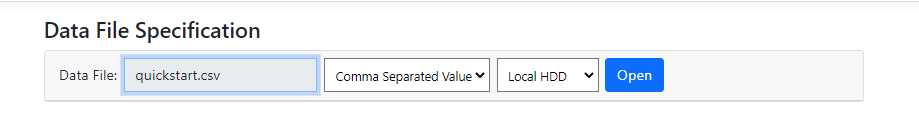
The Data page opens
Our data are in the CSV file quickstart.csv on a local
HDD, so click Select file to browse for this file:
Finally, note the trash can positioned in the top right
corner – to clear all input and start fresh, simply click on this icon.
Using the options above, we illustrate how to set up a
simple level-2 HLM model with 2 predictors from scratch. If you would like to
follow along, get the data here.
First, we need to select the data and specify which
variables to use. This is done on the landing page of the program.
To start, click New Analysis to start setting up a
new model.
The Data page opens
Our data are in the CSV file quickstart.csv on a local
HDD, so click Select file to browse for this file:
 The data in the file are displayed in the
first table on the updated Data page. To specify a model, information on
the structure of the data and the variables to be used in the analysis must be
supplied in the second table.
The data in the file are displayed in the
first table on the updated Data page. To specify a model, information on
the structure of the data and the variables to be used in the analysis must be
supplied in the second table.
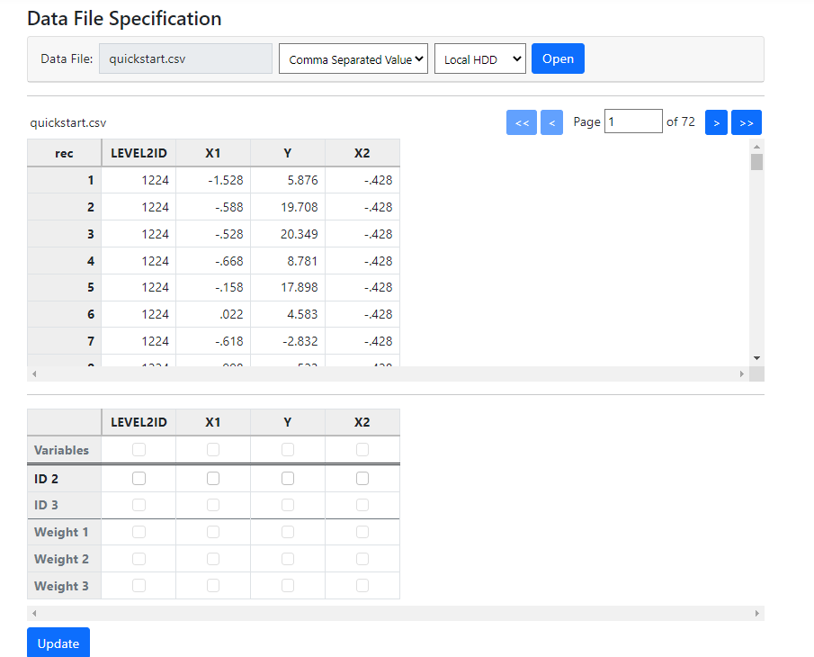 There are four variables:
-
LEVEL2ID defines the level-2 units
-
X1 is a potential predictor, as is X2
-
Y is the outcome variable
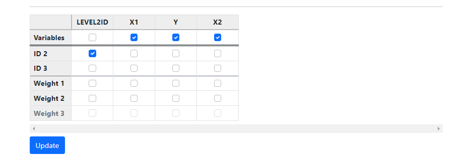
The levels of the hierarchical structure are captured in the
variable LEVEL2ID, so we select this as ID 2 by clicking the check box
for this variable in the ID 2 line. As we want to use all the other
variables in the model, we click the check boxes for all three in the Variables
line as showed below:
 Click Update, and the program will automatically
evaluate the levels of the variables and update the page to
Click Update, and the program will automatically
evaluate the levels of the variables and update the page to
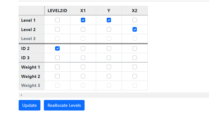 By comparing the allocation with the data in the first
table, we can see that X1 and Y are indeed level-1 variables, changing in value
from record to record. X2, on the other hand, has the same value for all
records with LEVEL2ID = 1224 and is correctly identified as a level-2 variable.
It is worth noting that the user can override this allocation by changing the
check boxes for the variables and clicking Update again. To reset
allocation to that determined by the program, the Reallocate Levels
button may be used. The Data page is now complete, and we click on Models
to start specifying the model.
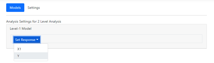
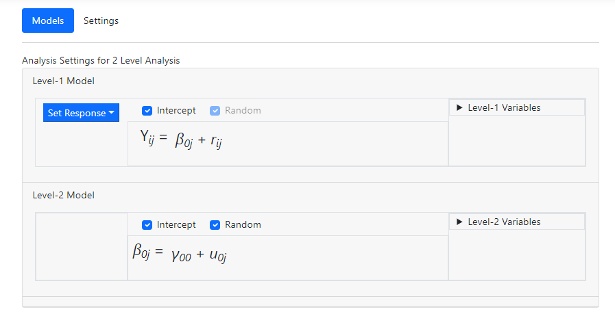
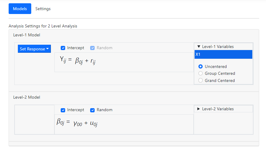
The Models page is now used to set up the model
equations.
The first step is to identify the outcome variable by
selecting Y from the drop-down list associated with the Set Response
option in the Level-1 model field as shown below.
The Models page is updated, displaying an
unconditional model with Y as outcome. Y is by default assumed to have both
fixed and random intercept coefficients. The model also includes a coefficient
for the residual variation at level-1.
By comparing the allocation with the data in the first
table, we can see that X1 and Y are indeed level-1 variables, changing in value
from record to record. X2, on the other hand, has the same value for all
records with LEVEL2ID = 1224 and is correctly identified as a level-2 variable.
It is worth noting that the user can override this allocation by changing the
check boxes for the variables and clicking Update again. To reset
allocation to that determined by the program, the Reallocate Levels
button may be used. The Data page is now complete, and we click on Models
to start specifying the model.
The Models page is now used to set up the model
equations.
The first step is to identify the outcome variable by
selecting Y from the drop-down list associated with the Set Response
option in the Level-1 model field as shown below.
The Models page is updated, displaying an
unconditional model with Y as outcome. Y is by default assumed to have both
fixed and random intercept coefficients. The model also includes a coefficient
for the residual variation at level-1.
 Next, the predictor X1 is added to the model by clicking on
the Level-1 Variables field. A variable can be entered in one of three
ways (uncentered, group mean centered or grand mean centered). Click on the
label X1 and drag it into the level-1 equation as uncentered predictor before
releasing the mouse.
Next, the predictor X1 is added to the model by clicking on
the Level-1 Variables field. A variable can be entered in one of three
ways (uncentered, group mean centered or grand mean centered). Click on the
label X1 and drag it into the level-1 equation as uncentered predictor before
releasing the mouse.
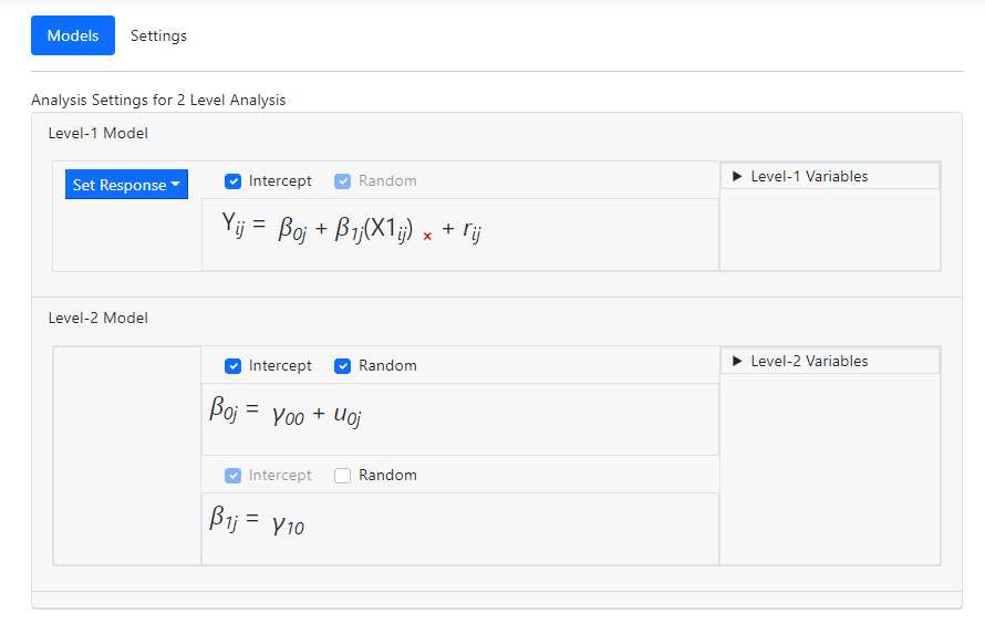
 The Models page updates to include a slope equation
for X1 at level-2.
The Models page updates to include a slope equation
for X1 at level-2.
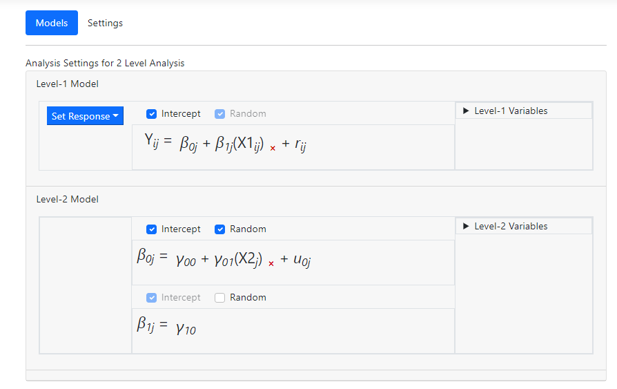
 Finally, add the level-2 predictor X2 to the intercept
equation using the Level-2 Variables field.
Finally, add the level-2 predictor X2 to the intercept
equation using the Level-2 Variables field.
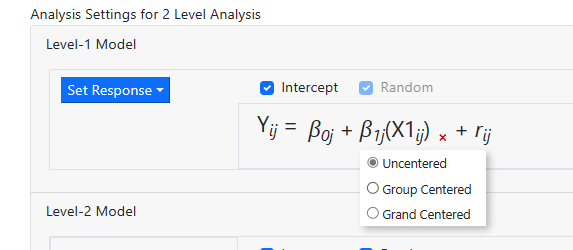
 Note that a variable may also be removed from the model by
simply clicking on the “x” next to
the variable name in the equation. The centering of a variable may also be
changed by moving the mouse over it to access the little pop-up menu below, on
which an alternative form of centering may be selected.
Note that a variable may also be removed from the model by
simply clicking on the “x” next to
the variable name in the equation. The centering of a variable may also be
changed by moving the mouse over it to access the little pop-up menu below, on
which an alternative form of centering may be selected.
 As our model is now complete, we can move on to specifying the
type of outcome variable we have using the Settings page.
As our model is now complete, we can move on to specifying the
type of outcome variable we have using the Settings page.
Specifying outcome distribution type and other options
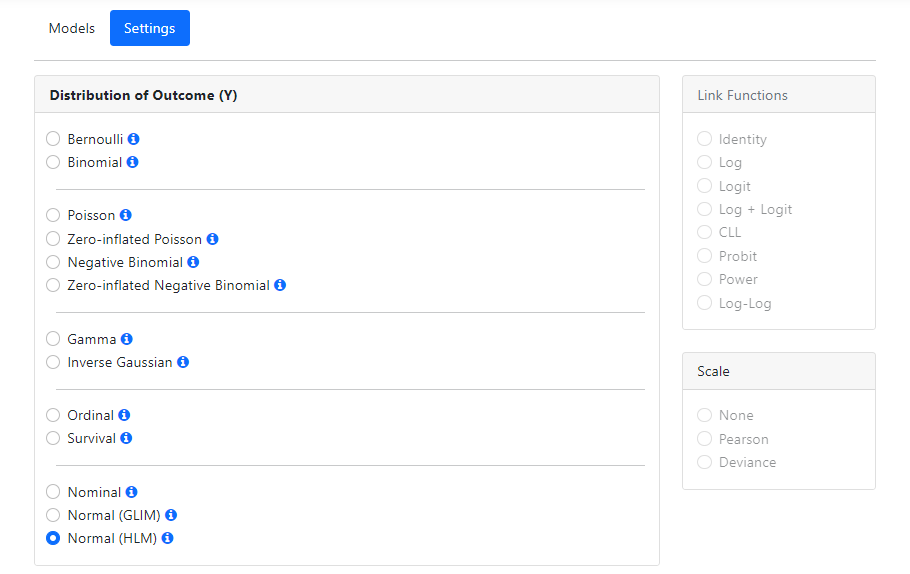
The basic model now complete, all that remains prior to
running the model is to specify the distribution type and other options (when
applicable). Click on Settings to access the Settings page.
The program will automatically select a distribution for the
outcome variable that it thinks most appropriate. Here, it selected Normal
(HLM), which is exactly what we want. As there are no other options that
need selecting, we can run the analysis. Click on Run at the top of the
page to go to the Run page.
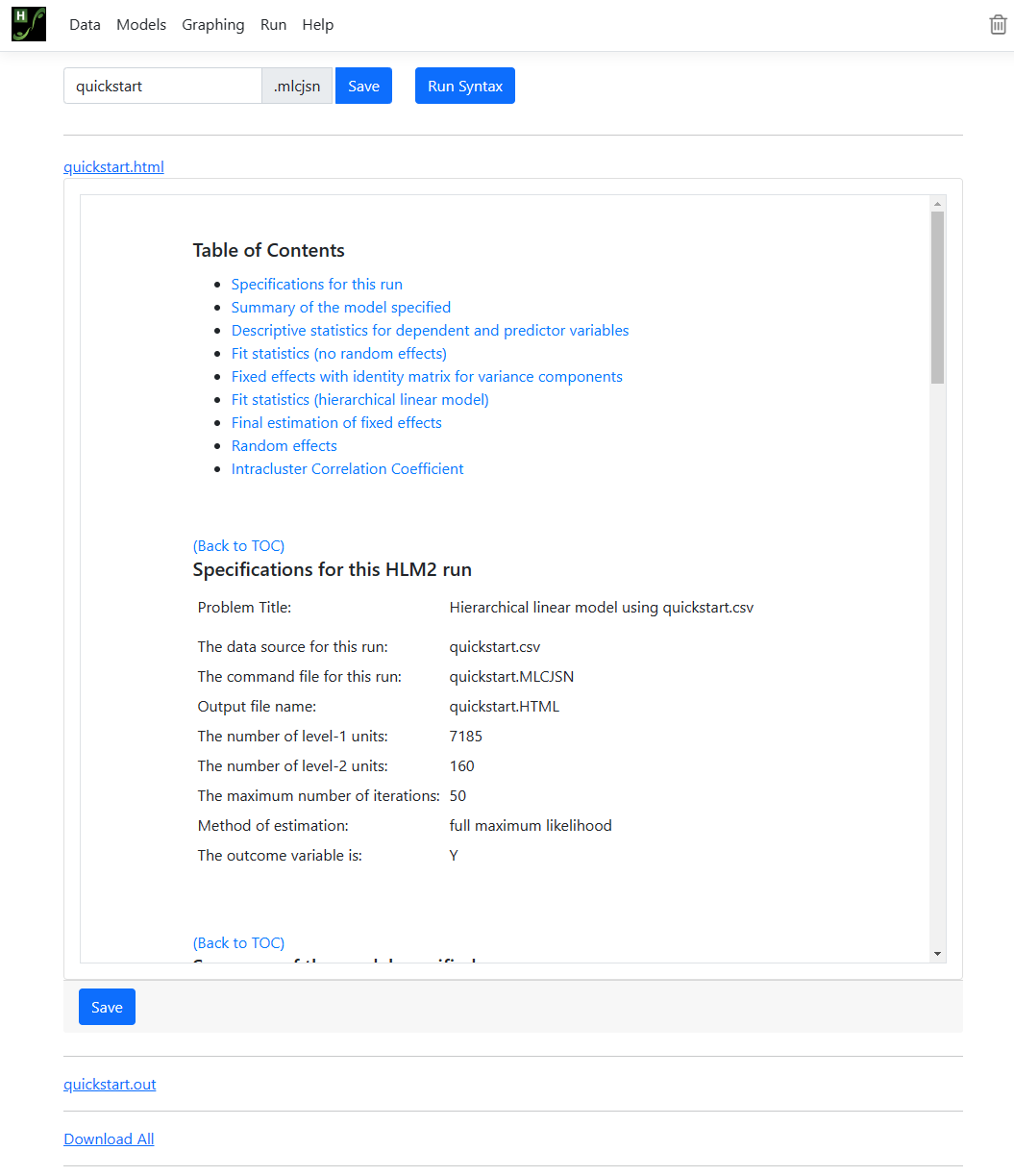
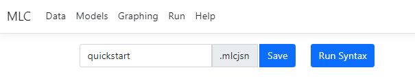
Run the analysis
The Run page is used to start the analysis, display
output in txt format and display graphs (when available).
For the current model, we can (optionally) save the model
information to a syntax file with MLCJSN file extension. By default, the file
name will correspond to that of the data file (quickstart, in this
case). Click Run Syntax to run the model.
A Progress box opens on the Run page,
displaying iterative information. Once complete, all output files are available for
viewing or downloading from the Run page.