Using the Settings page
The Settings page is used to specify the distribution
of the outcome variable. Link functions, as appropriate, are also selected here.
If a moderation analysis is to be performed, this page also allows selection
of focal and moderation variables.
The Settings page must be completed after completion of the Models
page, but before the Graphing or Syntax page is accessed.
Overview
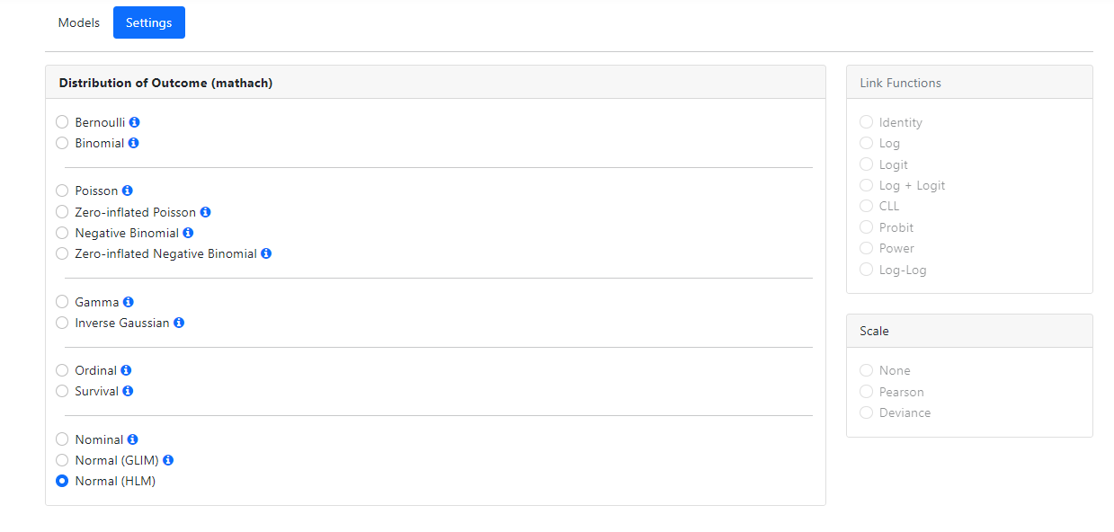
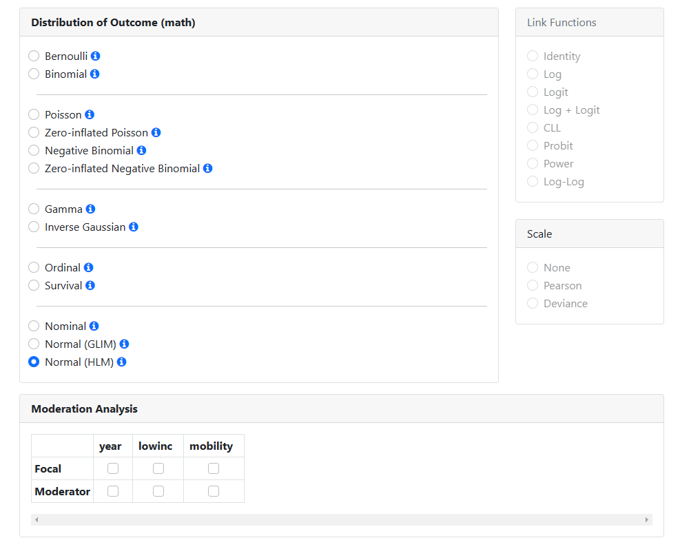
When first accessed, the program will suggest a suitable
distribution type based on its reading of the data. It is left to the user to
amend this should the suggested distribution not be appropriate. For example,
for data used here, the outcome is assumed to be a continuous normally
distributed variable, as indicated by the checked radio button next to the Normal
(HLM) option in the Distribution of Outcome field.
 Depending on the distribution selected, available additional
options such as link functions, scale, etc. will be activated for selection.
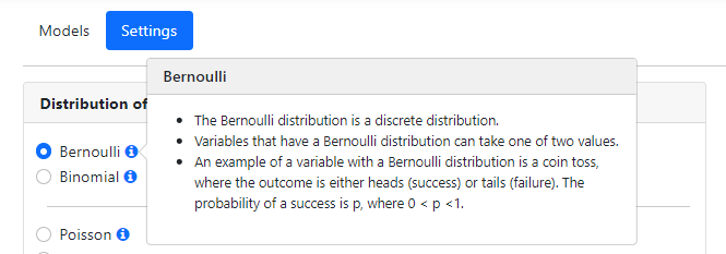
Note that by clicking on the “i” next to
a distribution type, basic information on the distribution type will be
displayed:
Depending on the distribution selected, available additional
options such as link functions, scale, etc. will be activated for selection.
Note that by clicking on the “i” next to
a distribution type, basic information on the distribution type will be
displayed:
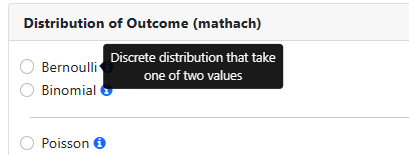
 For an even shorter description, simply move the mouse over
one of the items in the Distribution of Outcome field:
For an even shorter description, simply move the mouse over
one of the items in the Distribution of Outcome field:
Options available for distribution types
Descriptions and images showing the default option for each
distribution type are given here. To see the details for each, please select
from the list below. If you want the theory behind the model, visit our technical page.
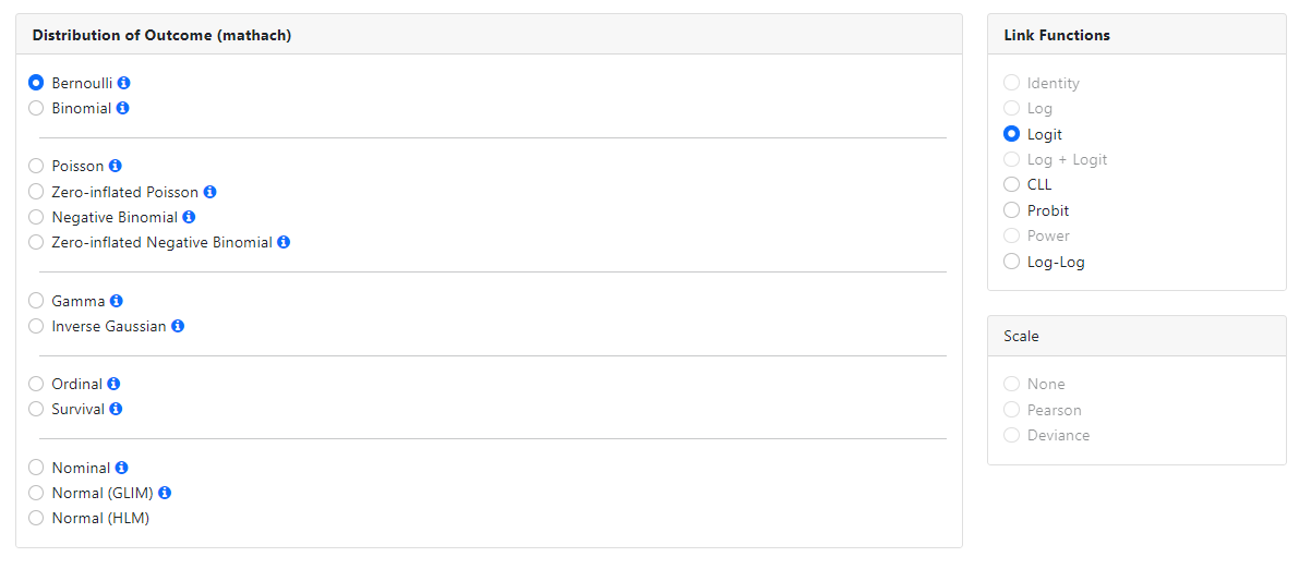
Bernoulli
The Bernoulli distribution is a discrete distribution.
Variables that have a Bernoulli distribution can take one of two values. An
example of a variable with a Bernoulli distribution is a coin toss, where the
outcome is either heads (success) or tails (failure). The probability of a
success is p, where 0 < p <1.
For the Bernoulli distribution, the logit, CLL, probit and
log-log link functions are available. The default link function is the logit
link.
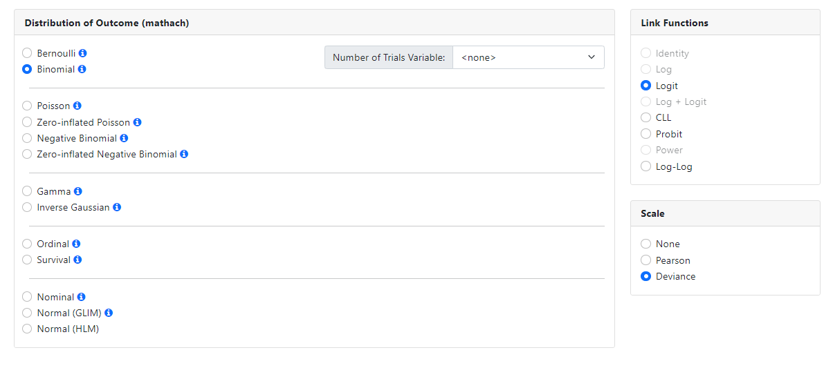
Binomial
The Binomial distribution is a discrete distribution in
which the outcome is binary. While the Bernoulli distribution is used to
describe the outcome of a single trial of an event, the Binomial
distribution is used when the outcome
of an event is observed multiple times.
For the Binomial distribution, the logit, CLL, probit and
log-log link functions are available. A Scale parameter can be
requested, with options being None, Pearson, or Deviance. The number of trials
is specified using the Number of Trials Variable field.
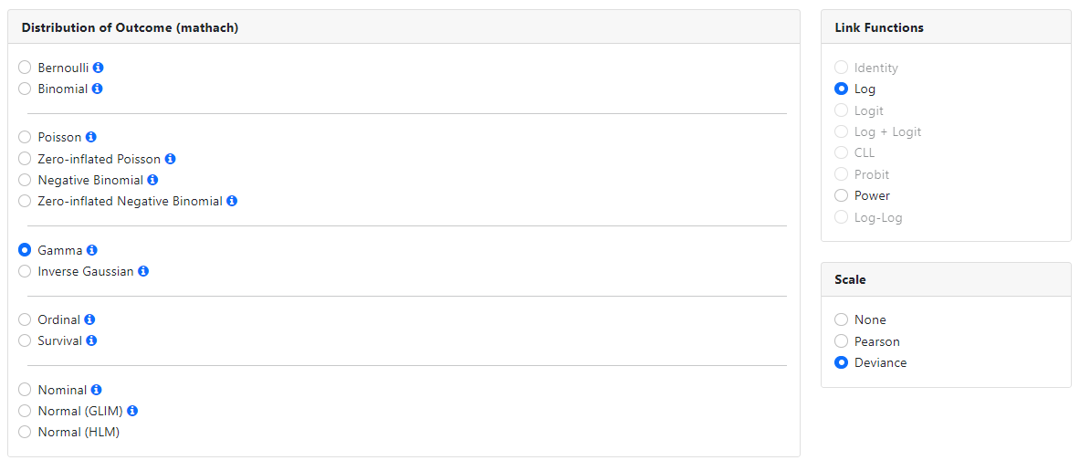
Gamma
The gamma distribution is a two-parameter continuous probability
distribution. It occurs when the waiting times between Poisson distributed
events are relevant.
A log or power link function may be specified, and a scale
parameter may be requested. By default, a log link function and the estimation
of a deviance scale parameter is assumed.
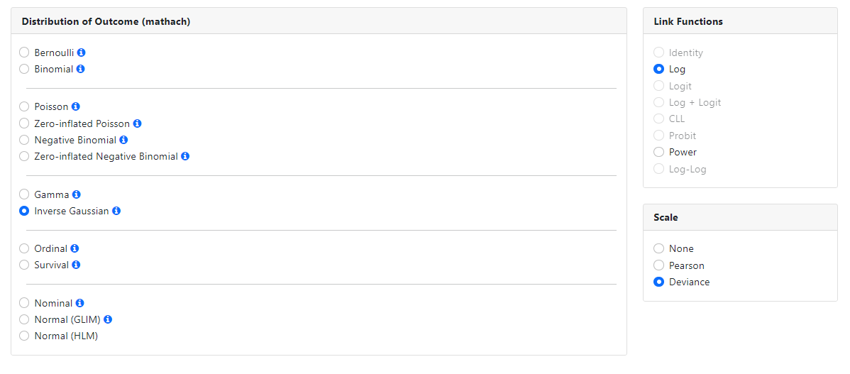
Inverse Gaussian
The inverse Gaussian distribution is a two-parameter family
of continuous probability distributions, first studied in relation to Brownian
motion. This distribution is one of a family of distributions that have been
called the Tweedie distributions, named after M.C.K. Tweedie who first used the
name Inverse Gaussian as there is an inverse relationship between the time to
cover a unit distance and distance covered in unit time.
A log or power link function may be specified, and a scale
parameter may be requested. By default, a log link function and the estimation
of a deviance scale parameter is assumed.
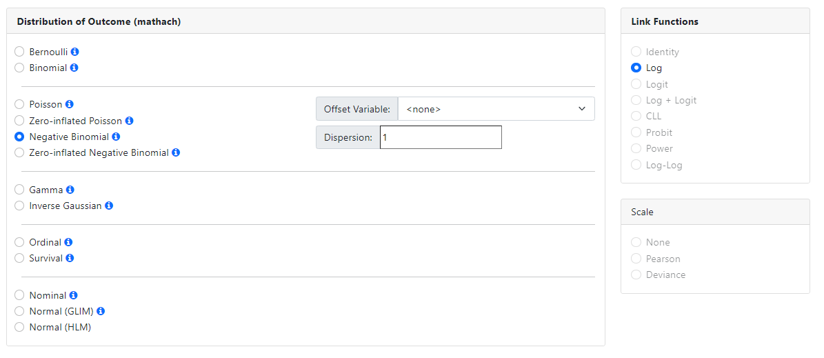
Negative Binomial
The negative binomial distribution is a discrete probability
distribution. It is used to model the number of successes in a sequence of
independent and identically distributed Bernoulli trials before a specified,
not random, number of failures occurs. The negative binomial model is an
extension of the Poisson model, in the sense that it adds a normally
distributed overdispersion effect.
For the negative binomial model, only a log link function is
available. A dispersion parameter (by default set to 1) and an offset variable
(if available) can also be specified.
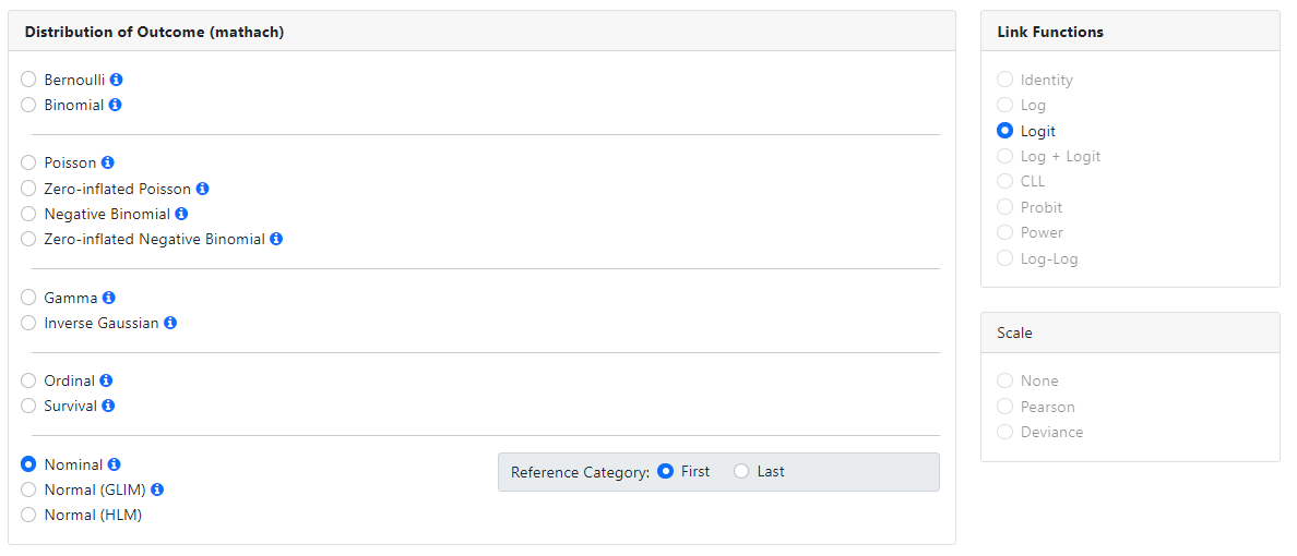
Nominal
The nominal model is part of a family of models based on the
multinomial distribution. The multinomial distribution is a generalization of
the Binomial distribution. It is commonly used in to describe the probability
of the outcome of n independent trials each of
which leads to a success for one of c categories, with each category
having a given fixed probability of success. A nominal variable has categories
that cannot be ordered.
A logit link function is used for a nominal outcome. By default,
it is assumed that the first category of the outcome should be used as
reference category, but this can also be set to the last category in the Reference
Category field.
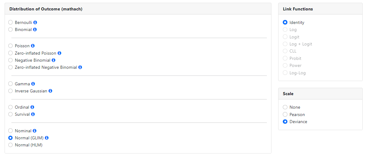
Normal distribution (GLIM)
Generalized linear
model (GLIM) for continuous normally distributed data. This model may be used
to check on the validity of the assumption of normality for a model run with
Normal (HLM). If the assumption of normality is reasonable, results should
correspond. If not, the inverse Gaussian and Gamma distributions should be
investigated as alternative distributions for the outcome variable.
When fitting a GLIM model to the data, the Identity link function is used. A scale parameter
may also be estimated.
Normal distribution (HLM)
When a hierarchical linear model, assuming a continuously
distributed outcome, is fitted to the data, the only additional option that may
be available is to specify a focal and moderator variable(s). The Moderation Analysis
field will only be activated if appropriate interaction terms appear in the
model specified.
If focal and moderator variable(s) are specified, the Graphing
page may be used to request simple slope and confidence interval plots.
Currently, graphing is only available for moderation analyses fitted after
selecting Normal (HLM) and completion of the Moderation Analysis field.
Full maximum likelihood estimation for continuous normally
distributed data. To check the validity of the assumption of normality, the
Normal (GLIM) distribution may be used.
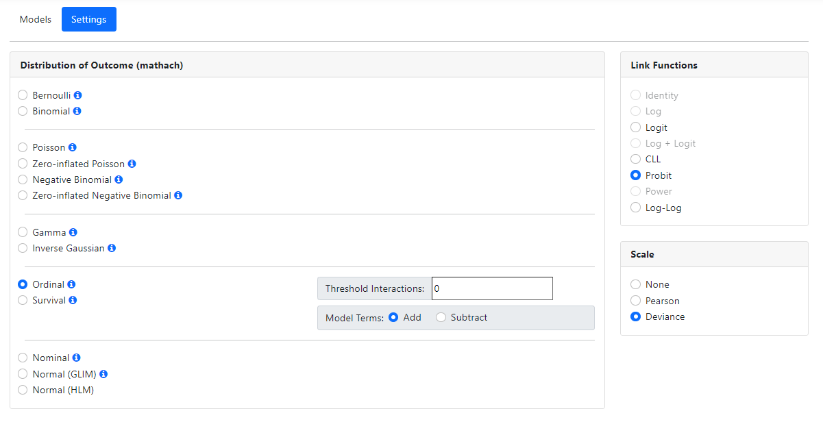
Ordinal
The ordinal model is also part of a family of models based
on the multinomial distribution. The multinomial distribution is a
generalization of the Binomial distribution. It is commonly used in to describe
the probability of the outcome of n
independent trials each of which leads to a success for one of c categories,
with each category having a given fixed probability of success. An ordinal
outcome is an outcome whose levels can be ordered.
For an analysis with ordinal outcome variable, the logit,
CLL, probit or log-log link functions may be specified. By default, a probit
link function is assumed, along with the estimated of a deviance
based scale parameter. Two additional options are available in this
case:
-
Threshold interactions may be requested. By default, no threshold interactions will
be estimated.
-
Model terms may be added or subtracted in the Model Terms field. By default,
adding of terms is assumed.
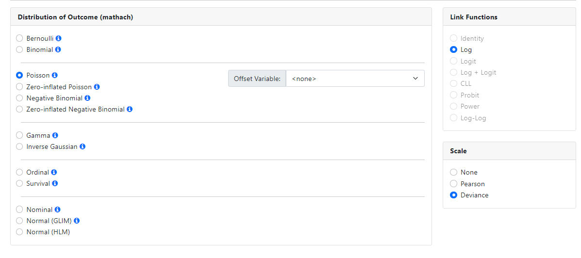
Poisson
The Poisson distribution is a discrete frequency
distribution that gives the probability of several independent events occurring
in a fixed time, given the average number of times the event occurs over that time period.
The Poisson model is fitted using a log link function. A
scale parameter may also be estimated. The Offset Variable field
may be used to specify the variable that denotes the exposure period.
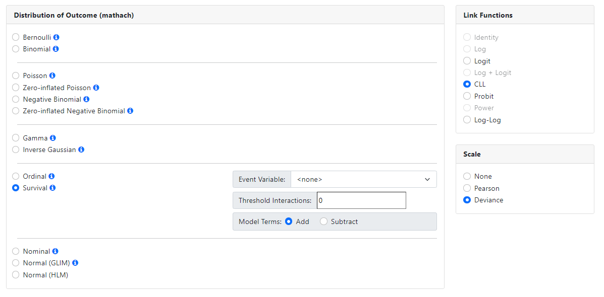
Survival analysis
The survival analysis model is used to describe the expected
duration of time until one or more events occur. Observations are censored, in
that for some units the event of interest did not occur during the entire time period studied. In addition, there may be predictors
whose effects on the waiting time need to be controlled or assessed.
The program makes provision for specifying a survival
analysis model as a separate model. Link functions available are the logit,
CLL, probit and log-log. The most commonly used link
function, CLL, is set as default. Additional options that may be specified are:
-
Scale parameter: By default set to Deviance
-
Event Variable:
Allows for the selection of a variable indicating whether the event in question
occurred at a time point.
-
Threshold interactions may be requested. By default, no threshold interactions will
be estimated.
-
Model terms may be added or subtracted in the Model Terms field. By default,
adding of terms is assumed.
Note that if the
user neglects to specify an Event Variable in the case of a survival
analysis, the analysis will stop with a warning message to this effect.
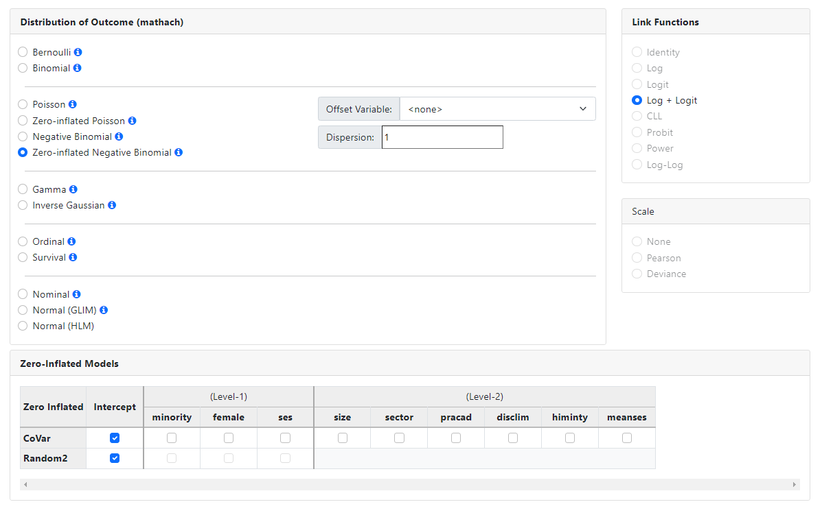
Zero-inflated negative binomial
The zero-inflated
negative Binomial model is a mixture model used to model count data that has an
excess of zero counts. It is assumed that the count in the not-always-zero
group has a negative binomial distribution.
The zero-inflated
model utilizes two link functions. The log link is used to model the negative
binomial model, and the logit link is used to model the excess of zeroes in the
outcome variable. A scale parameter may be estimated, and a dispersion
parameter (by default set to 1) may also be specified.
For the zero-inflated models, the Zero-Inflated Models field is activated. This
field is used to specify covariates and random effects for the logit component
of the mixed model, that is for the component modeling the excess of zeroes.
This allows the user to specify the basic negative binomial model on the Models
page, and the zero-inflated part through the Zero-Inflated Models field.
Variables to be included at either level of the hierarchy are selected by
simply checking the appropriate check box. By default, the logit model will be
estimated with only a fixed and random intercept, as shown in the image below.
Zero-inflated Poisson
The zero-inflated Poisson model is a mixture model used to
model count data that has an excess of zero counts. It is assumed that for
non-zero counts the counts are generated according to a Poisson model.
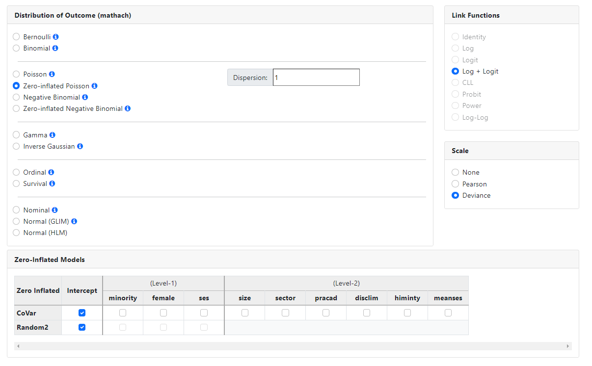
The ZIP model utilizes two link functions. The Log link is
used to model the Poisson model, and the logit link is used to model the excess
of zeroes in the outcome variable. A scale parameter may be estimated, and a
dispersion parameter (by default set to 1) may also be specified.
For the zero-inflated models, the Zero-Inflated Models
field is activated. This field is used to specify covariates and random effects
for the logit component of the mixed model, that is for the component modeling
the excess of zeroes. This allows the user to specify the basic Poisson model
on the Models page, and the zero-inflated part through the Zero-Inflated
Models field. Variables to be included at either level of the hierarchy are
selected by simply checking the appropriate check box. By default, the logit
model will be estimated with only a fixed and random intercept, as shown in the
image below.