Using the Models page
The Models page is used to specify the model to be
fitted. It consists of two parts, Models and Settings. The Settings
page is used to specify the type of outcome variable, link function (if
applicable) and other options for the analysis to be performed on the model as
set up on the Models page. The Models page must be completed
after completion of the Data page, but before the Settings page
is accessed.
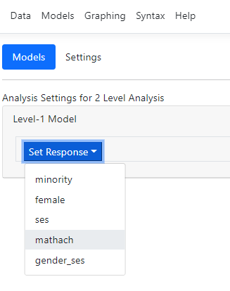
When the Models page is opened for the first time
after data specification, the only option available is the Set Response
option. This option is used to select the outcome variable from a drop-down
list containing all level-1 variables identified on the Data page. We
again use the familiar HS&B data to illustrate.
Setting up a model
The first step is to select the outcome/response variable
using the Set Response option:
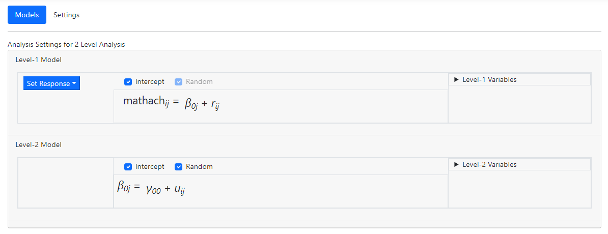
 After the outcome variable has been selected, the Models
page automatically updates to display an unconditional model where the selected
outcome variable MATHACH is modelled as having a fixed and random intercept, and allowance is
made for residual variation at level-1. Note that the model automatically
includes a fixed and random intercept, as indicated by the check marks in the
Intercept and Random check boxes. To remove a fixed or random effect, these
check boxes should be used.
Two new fields have been added to the right of the model: Level-1
Variables and Level-2 Variables. These are used to select predictors
at the respective levels and variables indicated as level-1 on the Data
page will appear on the list of Level-1 Variables, while level-2
variables will populate the Level-2 Variables list.
After the outcome variable has been selected, the Models
page automatically updates to display an unconditional model where the selected
outcome variable MATHACH is modelled as having a fixed and random intercept, and allowance is
made for residual variation at level-1. Note that the model automatically
includes a fixed and random intercept, as indicated by the check marks in the
Intercept and Random check boxes. To remove a fixed or random effect, these
check boxes should be used.
Two new fields have been added to the right of the model: Level-1
Variables and Level-2 Variables. These are used to select predictors
at the respective levels and variables indicated as level-1 on the Data
page will appear on the list of Level-1 Variables, while level-2
variables will populate the Level-2 Variables list.
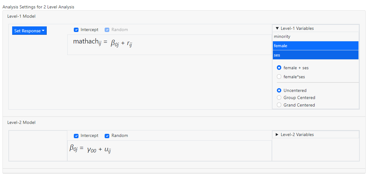
 We illustrate model building at level-1 by selecting the
variables FEMALE and SES to the level-1 equation. Click on the Level-1
Variables header and select the variables FEMALE and SES from the list,
holding down the Control or Shift key while doing so. The default
entry made by the program is now displayed: these two variables will be entered
as individual predictors (as indicated by the active option female + ses)
and they will be entered uncentered (again, as indicated by the default
value displayed below).
We illustrate model building at level-1 by selecting the
variables FEMALE and SES to the level-1 equation. Click on the Level-1
Variables header and select the variables FEMALE and SES from the list,
holding down the Control or Shift key while doing so. The default
entry made by the program is now displayed: these two variables will be entered
as individual predictors (as indicated by the active option female + ses)
and they will be entered uncentered (again, as indicated by the default
value displayed below).
 Drag the selected variables into the level-1 equation.
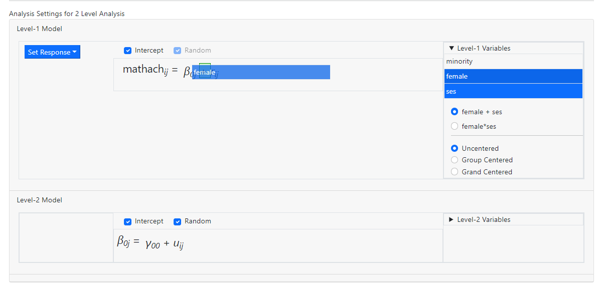 to obtain the model
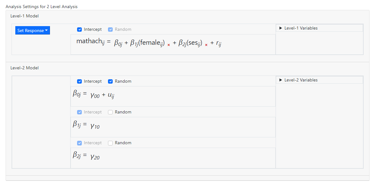 Note that fixed slope effects for the two predictors have
been added at level-2 of the model. By default, slopes are assumed fixed. To
allow a slope to vary randomly, check the Random box in the relevant
slope equation.
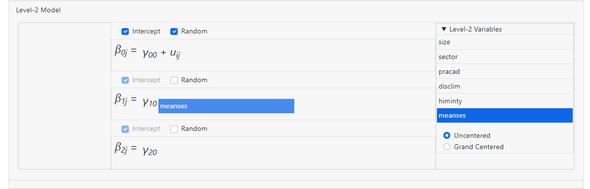
Level-2 model building is done in the same way. For example,
an uncentered fixed effect for the level-2 variable MEANSES is added to the
slope equation of gender (as represented by the level-1 variable FEMALE) in the
image below.
Note that fixed slope effects for the two predictors have
been added at level-2 of the model. By default, slopes are assumed fixed. To
allow a slope to vary randomly, check the Random box in the relevant
slope equation.
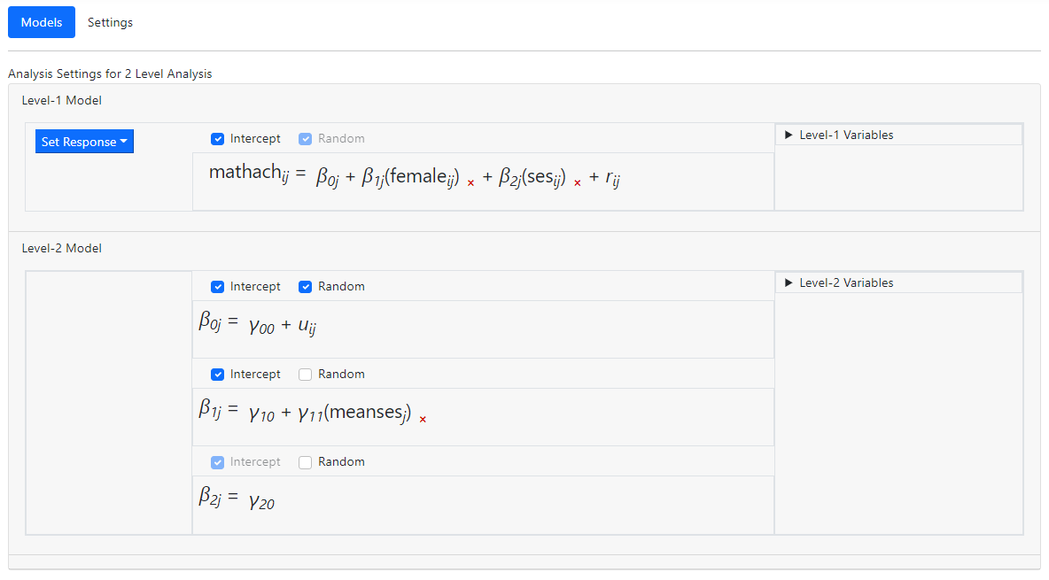
Level-2 model building is done in the same way. For example,
an uncentered fixed effect for the level-2 variable MEANSES is added to the
slope equation of gender (as represented by the level-1 variable FEMALE) in the
image below.
 resulting in the model
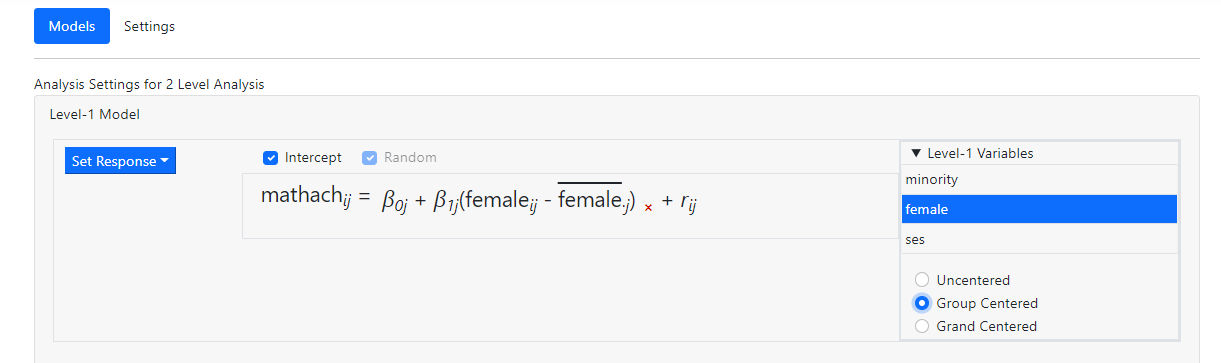
 In the example above, all variables were entered into the
model as uncentered models. Variables may also be entered as group-mean or
grand-mean centered.
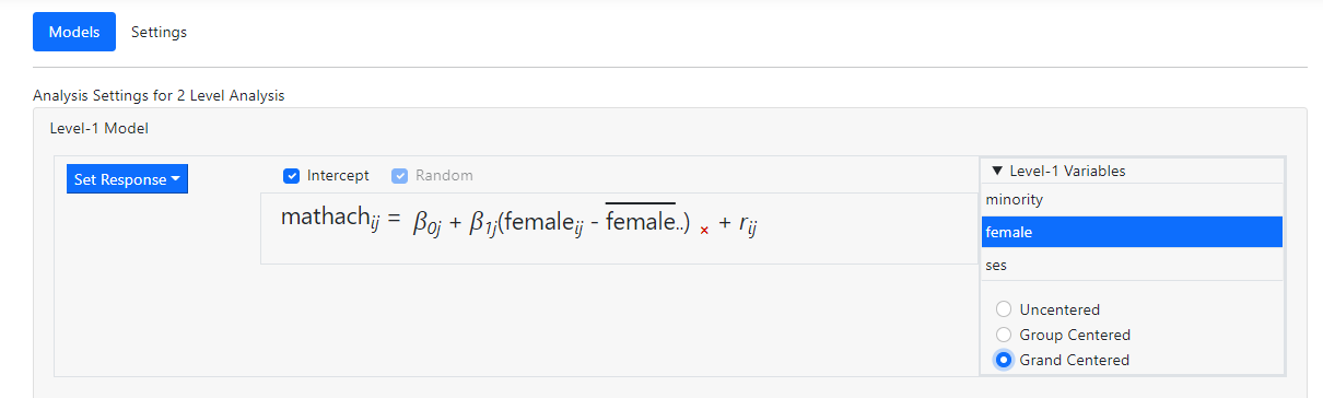
The image below shows the inclusion of female as group-mean
centered variable. The notation used in the equation for this variable
indicates that the group mean for a given group j is subtracted from the
values of his variables for all level-1 observations nested within group j.
In the example above, all variables were entered into the
model as uncentered models. Variables may also be entered as group-mean or
grand-mean centered.
The image below shows the inclusion of female as group-mean
centered variable. The notation used in the equation for this variable
indicates that the group mean for a given group j is subtracted from the
values of his variables for all level-1 observations nested within group j.
 In the case of grand mean centering, the mean over all
observations, irrespective of the level-2 unit they belong to, is subtracted as
reflected in the notation shown in the image below.
In the case of grand mean centering, the mean over all
observations, irrespective of the level-2 unit they belong to, is subtracted as
reflected in the notation shown in the image below.
 After completing the Models page, the Settings
page is used to specify the type of outcome variable and select options
available for the selected type of outcome variable.
After completing the Models page, the Settings
page is used to specify the type of outcome variable and select options
available for the selected type of outcome variable.
How do I create a same-level interaction?
It is not necessary to create same-level interactions prior
to importing the data into the program. The program allows the user to create
interaction terms on the fly. Same level interactions are specified during the
model specification, using the Models page.
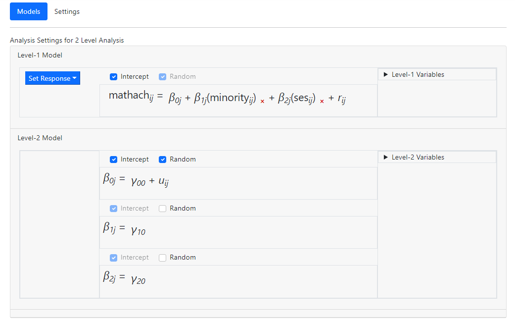
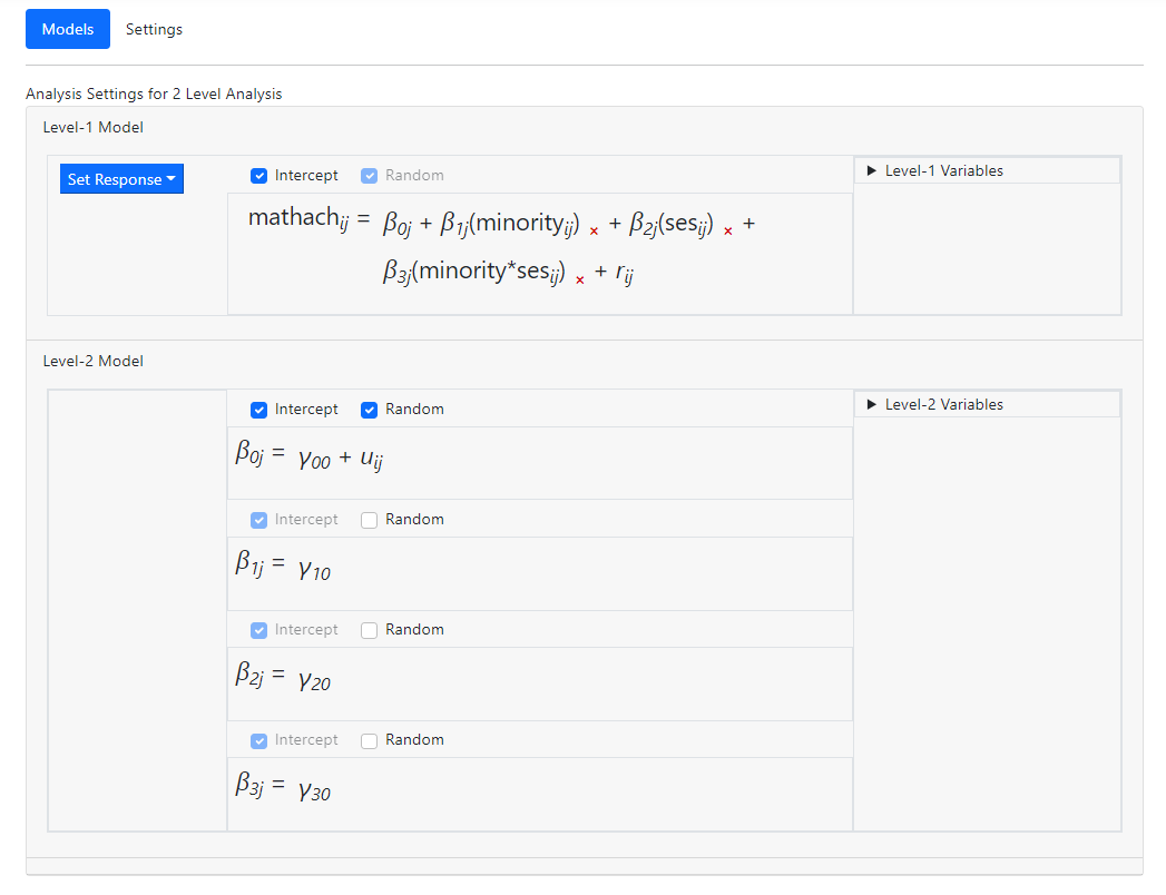
Consider the following random-intercept-only model modelling
a student’s math achievement (MATHACH) as a function of the predictors
MINORITY and SES.
 Suspecting that there may be a significant interaction
between these predictors, we wish to add a same level interaction term. To do
so, we open the Level-1 Variables list and, holding the Control
key down, select both variables
Suspecting that there may be a significant interaction
between these predictors, we wish to add a same level interaction term. To do
so, we open the Level-1 Variables list and, holding the Control
key down, select both variables
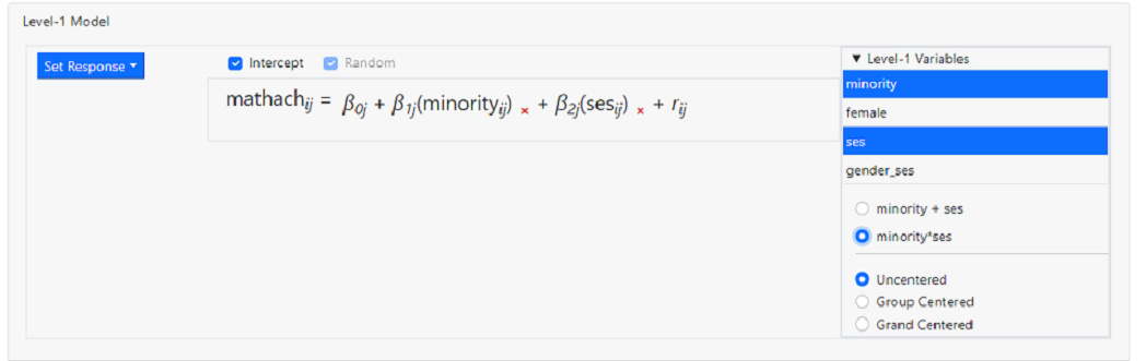 Notice that, by default, these variables will be entered as Uncentered.
In addition, the program allows us to add multiple variables in one of two
ways:
Notice that, by default, these variables will be entered as Uncentered.
In addition, the program allows us to add multiple variables in one of two
ways:
-
Minority + ses: selecting this option
will add the selected variables as individual predictors into the level-1
model. This is the default selection.
-
Minority*ses: selecting this option will
add an interaction between the two selected variables into the level-1 model.
As the setting minority*ses is what we want, we click
the radio button next to this option and simply drag the selected variables
into the level-1 equation
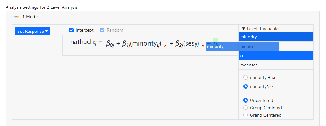 before releasing the mouse. Once the term has been dropped,
the model becomes
before releasing the mouse. Once the term has been dropped,
the model becomes
 The fixed effect in the last of the level-2 equations represents the same-level
interaction between the two level-1 variables MINORITY and SES.
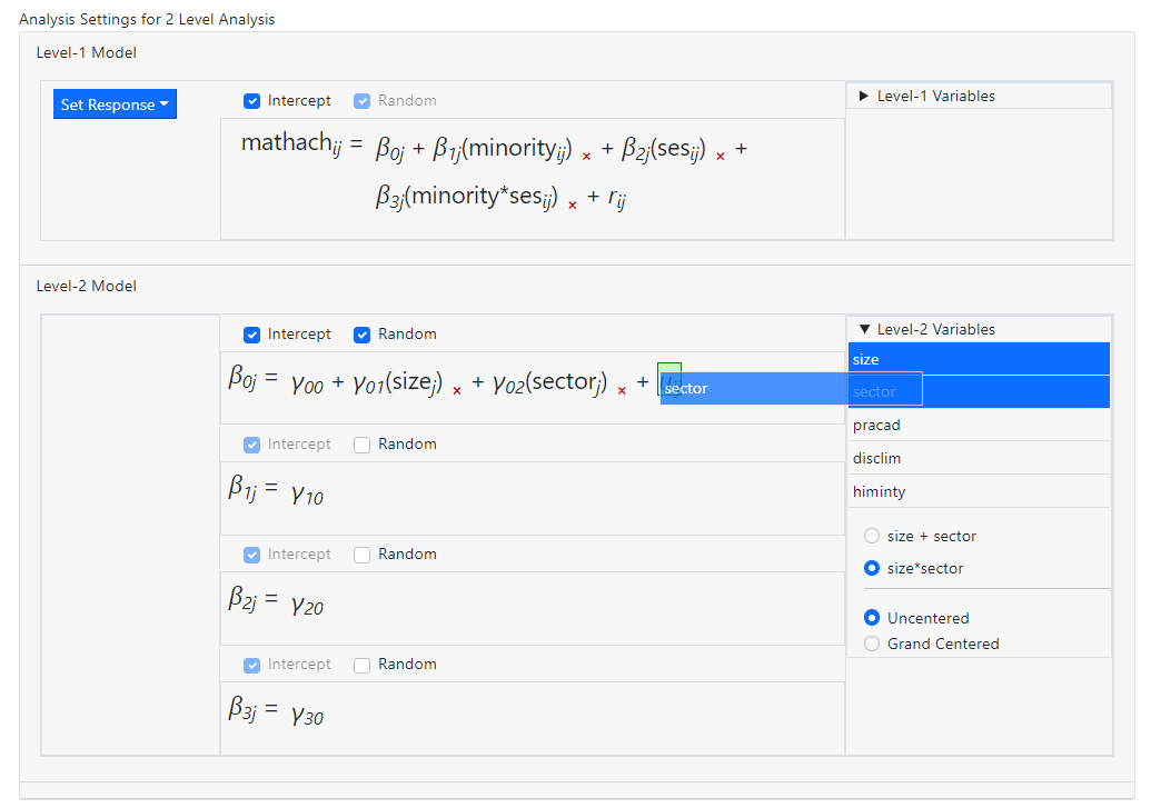
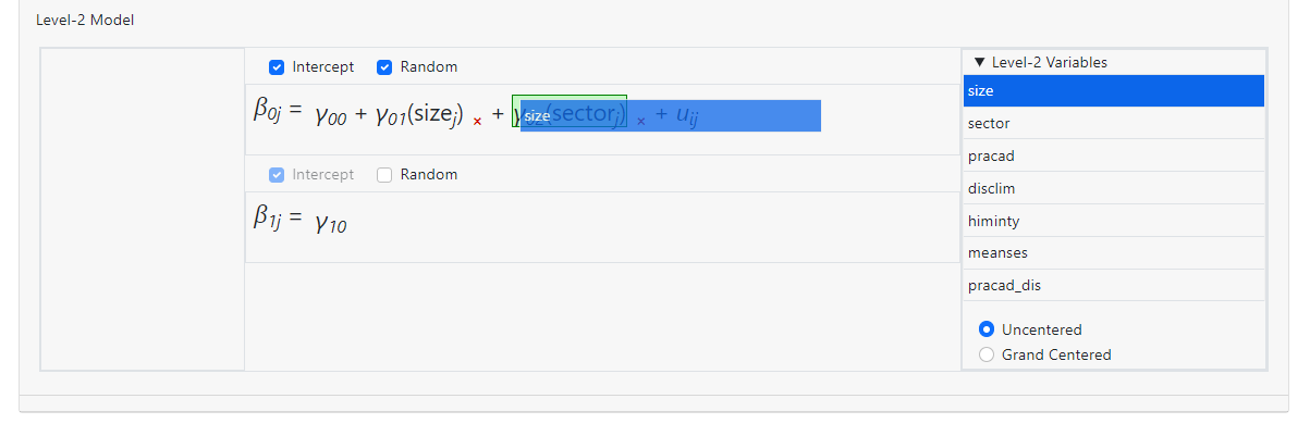
It is also possible to add same-level interactions at a
higher level. In the example below, an interaction term between the variables
SIZE and SECTOR is being added to the first of the level-2 equations.
The fixed effect in the last of the level-2 equations represents the same-level
interaction between the two level-1 variables MINORITY and SES.
It is also possible to add same-level interactions at a
higher level. In the example below, an interaction term between the variables
SIZE and SECTOR is being added to the first of the level-2 equations.
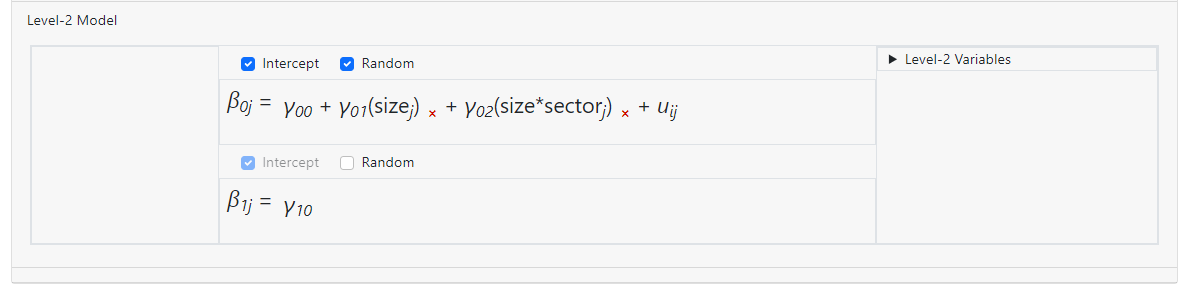
 After dropping these into the model, the equation in question becomes
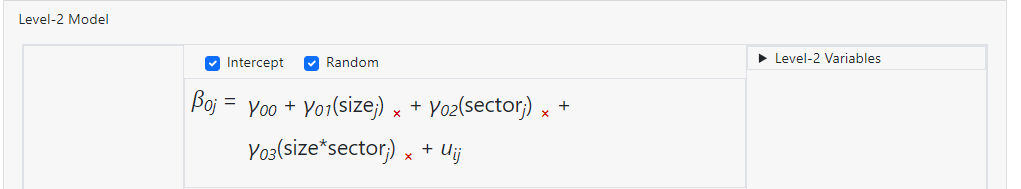 and
and  is
the fixed coefficient associated with the interaction term.
A single predictor may also be dragged on top of a predictor
already in the model before releasing the mouse, creating an interaction term
that way. When that is done, however, note that the predictor previously in the
model is no longer present in the same form as before and if required, would
have to be added back into the model.
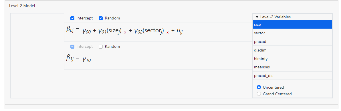
In the model below, the predictors SIZE and SECTOR are already in the model:
is
the fixed coefficient associated with the interaction term.
A single predictor may also be dragged on top of a predictor
already in the model before releasing the mouse, creating an interaction term
that way. When that is done, however, note that the predictor previously in the
model is no longer present in the same form as before and if required, would
have to be added back into the model.
In the model below, the predictors SIZE and SECTOR are already in the model:
 Dragging the variable SIZE on top of SECTOR as shown below
 creates a model with a two-way interaction size*sector,
but there is no longer an individual coefficient for the variable SECTOR in the
equation.
creates a model with a two-way interaction size*sector,
but there is no longer an individual coefficient for the variable SECTOR in the
equation.
How many interactions can be included in the model?
The maximum number of interactions allowed in the program is
a 3-way interaction, in other words, an interaction of the form a*b*c. There
are no limits on the number of individual 2-way or 3-way interactions.
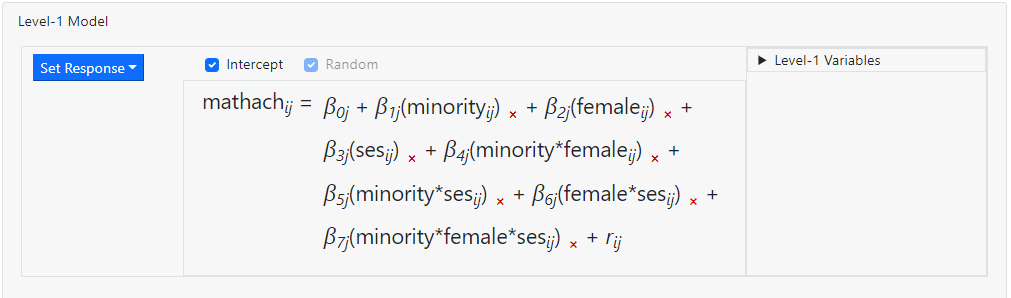
In the level-1 model below, three predictors have been
entered. 2-way Interactions between all possible pairs of the variables are
also present in the model (for example minority*ses), along with
a 3-way interaction (minority*female*ses). While it is
possible to add more than 3 predictors simultaneously, selecting more than
three variables at the same time will disable the option on the Level-1
Variables box that allows for creating an interaction effect.
 Turning to higher-levels, the type of interaction that can be
added to the model depends on the equation the selection is to be added to.
Turning to higher-levels, the type of interaction that can be
added to the model depends on the equation the selection is to be added to.
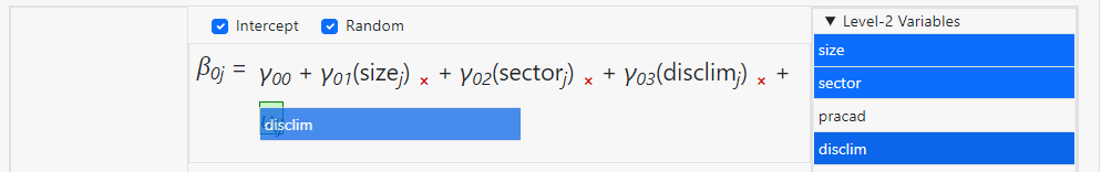
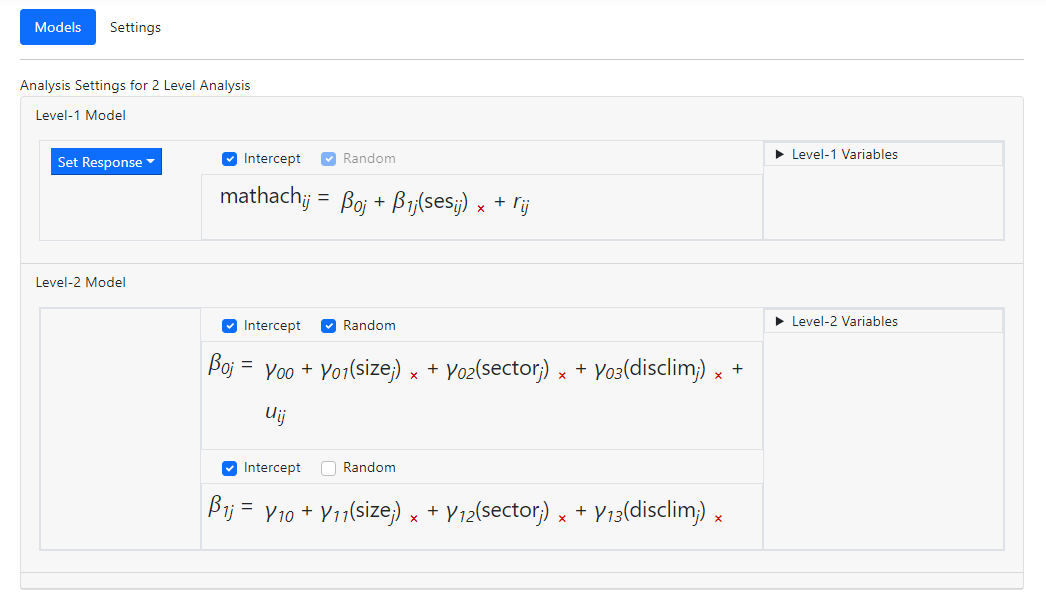 Suppose we would like to add an interaction term to the two
level-2 equations. In the case of the first equation, a three-way interaction
term of the form size*sector*disclim may be added
Suppose we would like to add an interaction term to the two
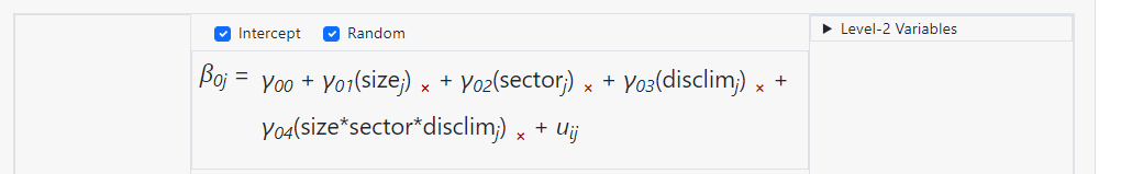
level-2 equations. In the case of the first equation, a three-way interaction
term of the form size*sector*disclim may be added
 to obtain the equation
 When we attempt to add a similar term to the second level-2
equation, the program does not allow this. When we drag the interaction term
into the equation, an
When we attempt to add a similar term to the second level-2
equation, the program does not allow this. When we drag the interaction term
into the equation, an  image
appears, indicating that this is not allowed.
Why the difference in behavior? The answer lies in the fact
that
image
appears, indicating that this is not allowed.
Why the difference in behavior? The answer lies in the fact
that  is the intercept
equation, but
is the intercept
equation, but  is a slope
equation.
If we substitute the
is a slope
equation.
If we substitute the  into the
level-1 equation, we obtain
into the
level-1 equation, we obtain
 However, if we could do the same with
  , we would get
 and the last term,
  , would be a four-way interaction.
Although the same
level-2 variables appear on the two level-2 equations, those on the equation
for are already multiplied
with the values of the level-1 predictor SES. This implies that for this
equation, only 2-way interaction terms may be added so as not to exceed the
program limit of maximum three terms a*b*c. If we had managed to add the
three-way interaction to the second equation, we would in effect have added a
4-way interaction of the form a*b*c*d.
Apart from the 3-way interaction limit, there is no limit on
the number of individual 2- or 3-way interaction terms that can be added to the
model. In other words, a model with 10 2-way interactions and 4 3-way
interactions would, theoretically be possible, if somewhat inadvisable in terms
of estimation.
, would be a four-way interaction.
Although the same
level-2 variables appear on the two level-2 equations, those on the equation
for are already multiplied
with the values of the level-1 predictor SES. This implies that for this
equation, only 2-way interaction terms may be added so as not to exceed the
program limit of maximum three terms a*b*c. If we had managed to add the
three-way interaction to the second equation, we would in effect have added a
4-way interaction of the form a*b*c*d.
Apart from the 3-way interaction limit, there is no limit on
the number of individual 2- or 3-way interaction terms that can be added to the
model. In other words, a model with 10 2-way interactions and 4 3-way
interactions would, theoretically be possible, if somewhat inadvisable in terms
of estimation.