FAQ: (GUI)
Common questions regarding use of the GUI are addressed in the following topics:
What kind of input files can I use?
What to do if variables are assigned incorrectly?
What output files can I get?
How do I create a same-level interaction?
How do I remove variables or change their centering options?
What graphs can I get?
Can graphs be modified?
How do I center variables?
How many interactions can be included in the model?
Explanation of error messages (GUI)
What kind of input files can I use?
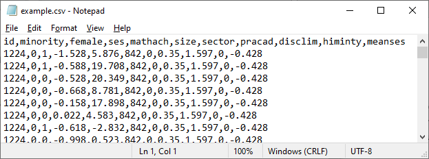
Currently,
only CSV files are supported. Here is an example of a Comma separated Value
(*.csv file extension) file:
 The Data page is used to read in data. Click on Select file to open
an Open dialog box to select a data file.
The Data page is used to read in data. Click on Select file to open
an Open dialog box to select a data file.
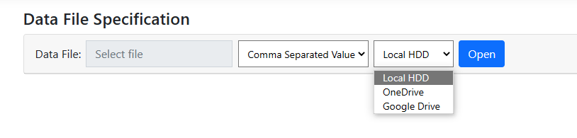 By default, it is assumed that the data file is on the local hard drive disk
(Local HDD). However, one may also use an URL, OneDrive of Google
Drive to select the file from.
Once the file name,
type and location has been specified, click Open to display the contents
of the data file.
By default, it is assumed that the data file is on the local hard drive disk
(Local HDD). However, one may also use an URL, OneDrive of Google
Drive to select the file from.
Once the file name,
type and location has been specified, click Open to display the contents
of the data file.
What to do if variables are assigned incorrectly?
Once variables are selected on the Data page, clicking the Update button prompts the
program to automatically determine the appropriate level of the hierarchy each
variable is associated with. Sometimes, however, problems can occur. To
illustrate, consider the following example, based on the well-known HS&B
data, in which students are nested with schools and we have information on the
mean socio-economic status of each school represented by the variable MEANSES.
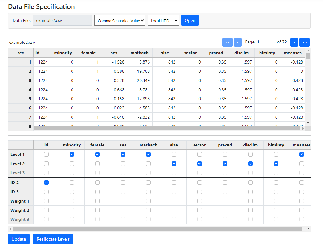 In this case, the
program assigned the variable MEANSES to level-1. This is surely incorrect, as
we know it to be a school rather than a student characteristic.
Inspection of the
data in the first table for this variable shows that, instead of having the
same value for MEANSES for all students within school with ID 1224 as would be
expected of a school-level variable, the data for the second student (second
record) shows a value of 0. This means that the values of this variable change
within a school over students, and do not remain constant for all students
within the school as a true level-2 variable should. This is most likely a data
entry error and the best solution would be to clean the data and inspect it for
similar problems with other variables.
However, the program
allows the user to override program allocation without editing the data. If a
user wishes to proceed regardless, the level-1 check box for MEANSES can be
unchecked and the level-2 check box can be checked instead. Clicking the Update
button again will retain this modification. In effect, the program respects the
user’s opinion.
Should the user
prefer the program’s allocation at a later stage, clicking Reallocate
Levels will reset the level allocation to the initial automatic allocation
performed by the program.
In this case, the
program assigned the variable MEANSES to level-1. This is surely incorrect, as
we know it to be a school rather than a student characteristic.
Inspection of the
data in the first table for this variable shows that, instead of having the
same value for MEANSES for all students within school with ID 1224 as would be
expected of a school-level variable, the data for the second student (second
record) shows a value of 0. This means that the values of this variable change
within a school over students, and do not remain constant for all students
within the school as a true level-2 variable should. This is most likely a data
entry error and the best solution would be to clean the data and inspect it for
similar problems with other variables.
However, the program
allows the user to override program allocation without editing the data. If a
user wishes to proceed regardless, the level-1 check box for MEANSES can be
unchecked and the level-2 check box can be checked instead. Clicking the Update
button again will retain this modification. In effect, the program respects the
user’s opinion.
Should the user
prefer the program’s allocation at a later stage, clicking Reallocate
Levels will reset the level allocation to the initial automatic allocation
performed by the program.
What output files
can I get?
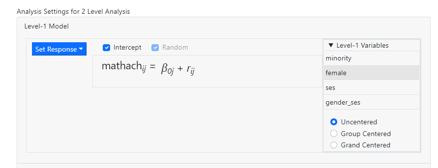
Results of the analysis are available from the Run page via links. Both HTML and standard txt file output are available. Moderation graphs, if requested, are also given here. In addition, all relevant files, from data to syntax to output, can be downloaded by clicking on the Download All link.
This option is particularly useful should you want to rerun the analysis at a later date.
How do I create a same-level interaction?
It is not necessary
to create same-level interactions prior to importing the data into the program.
The program allows the user to create interaction terms on the fly. Same level
interactions are specified during the model specification, using the Models
page.
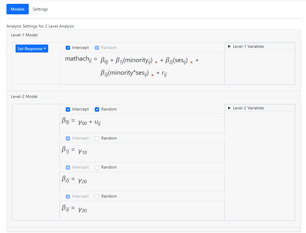
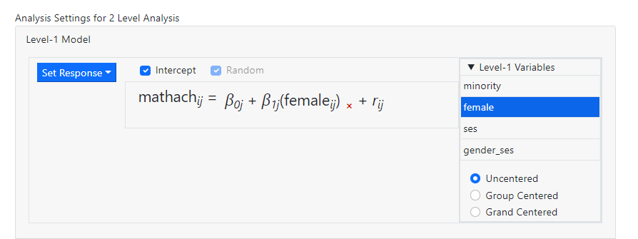
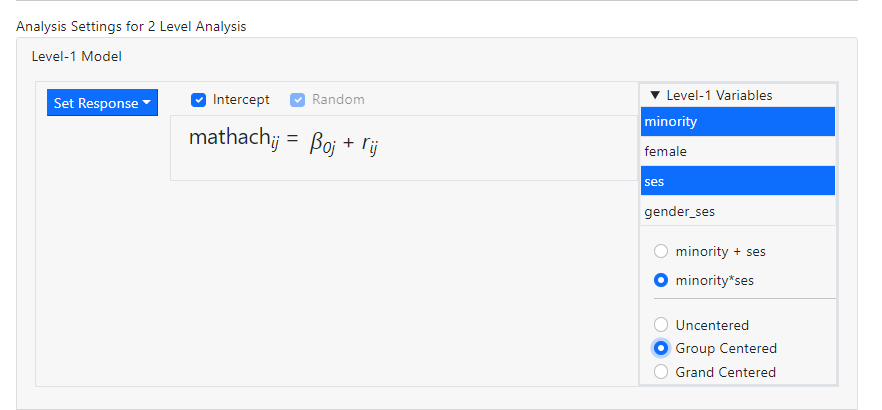
Consider the following
random-intercept-only model modelling a student’s math achievement
(MATHACH) as a function of the predictors MINORITY and SES.
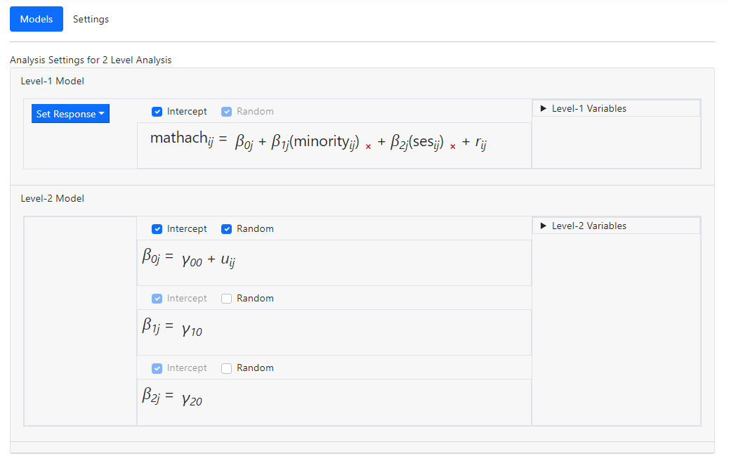 Suspecting that
there may be a significant interaction between these predictors, we wish to add
a same level interaction term. To do so, we open the Level-1 Variables
list and, holding the Control key down, select both variables.
Suspecting that
there may be a significant interaction between these predictors, we wish to add
a same level interaction term. To do so, we open the Level-1 Variables
list and, holding the Control key down, select both variables.
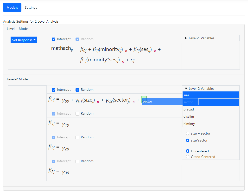
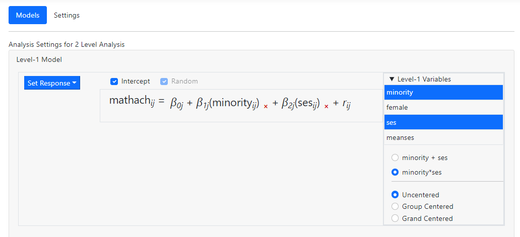 Notice that, by
default, these variables will be entered as Uncentered. In addition, the
program allows us to add multiple variables in one of two ways:
Notice that, by
default, these variables will be entered as Uncentered. In addition, the
program allows us to add multiple variables in one of two ways:
-
Minority + ses: selecting this option will add the selected
variables as individual predictors into the level-1 model. This is the default
option.
-
Minority*ses: selecting this option will add an interaction between the
two selected variables into the level-1 model.
As the setting minority*ses
is exactly what we want, we click the radio button next to this option, and
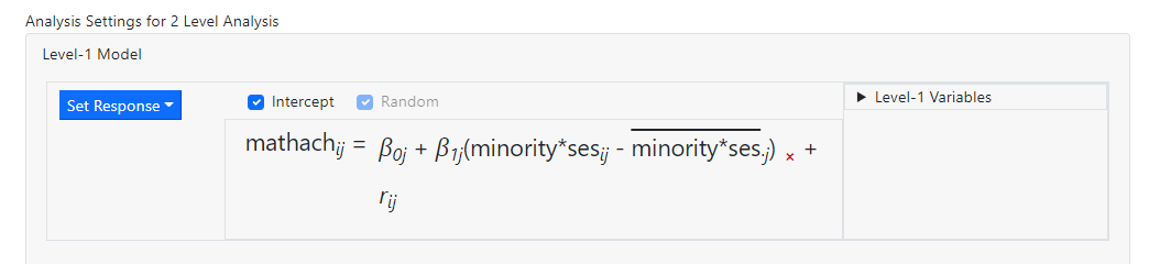
simply drag the selected variables into the level-1 equation
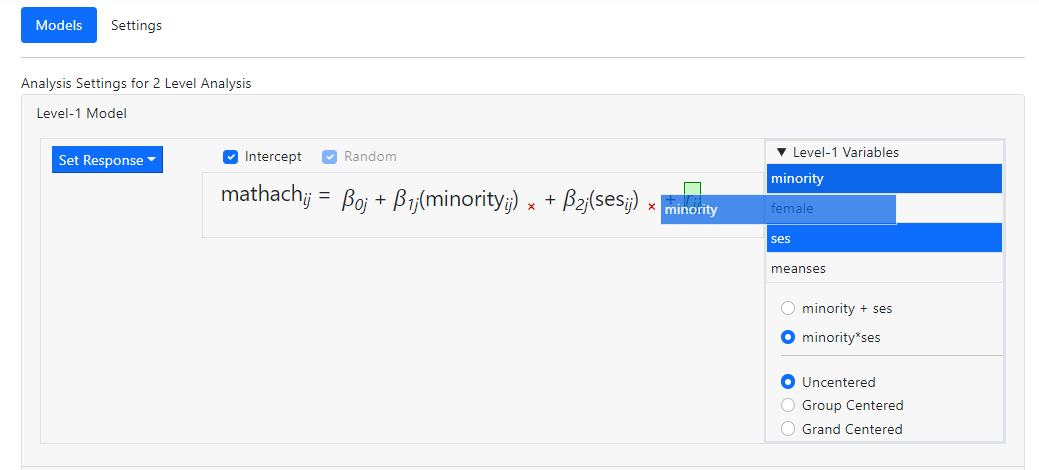 before releasing the
mouse. Once the term has been dropped, the model becomes
before releasing the
mouse. Once the term has been dropped, the model becomes
 The fixed effect
  in the
  equation
represents the same-level interaction between the two level-1 variables
MINORITY and SES.
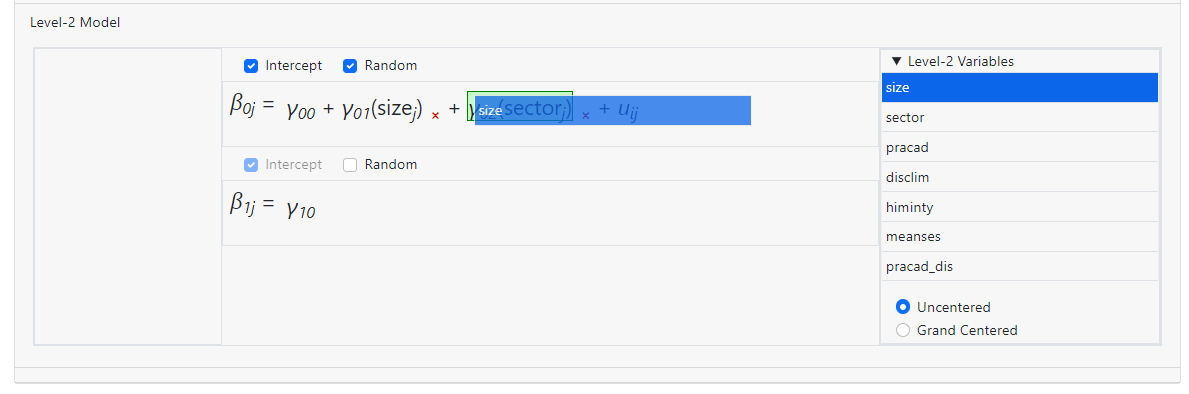
It is also possible to
add same-level interactions at a higher level. In the example below, an
interaction term between the variables SIZE and SECTOR is being added to the
first of the level-2 equations.
equation
represents the same-level interaction between the two level-1 variables
MINORITY and SES.
It is also possible to
add same-level interactions at a higher level. In the example below, an
interaction term between the variables SIZE and SECTOR is being added to the
first of the level-2 equations.
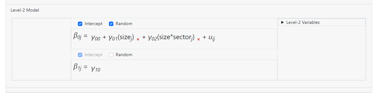
 After dropping these
into the model, the equation in question becomes
After dropping these
into the model, the equation in question becomes
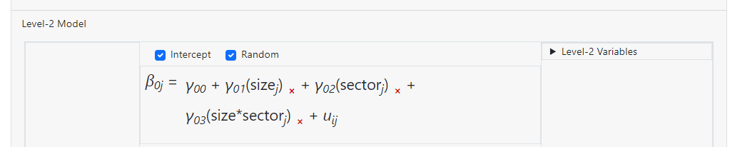 and
and  is the fixed
coefficient associated with the interaction term.
A single predictor
may also be dragged on top of a predictor already in the model before releasing
the mouse, creating an interaction term that way. When that is done, however,
note that the predictor previously in the model is no longer present in the
same form as before and if required, would have to be added back into the
model.
In the model below,
the predictors SIZE and SECTOR are already in the model:
is the fixed
coefficient associated with the interaction term.
A single predictor
may also be dragged on top of a predictor already in the model before releasing
the mouse, creating an interaction term that way. When that is done, however,
note that the predictor previously in the model is no longer present in the
same form as before and if required, would have to be added back into the
model.
In the model below,
the predictors SIZE and SECTOR are already in the model:
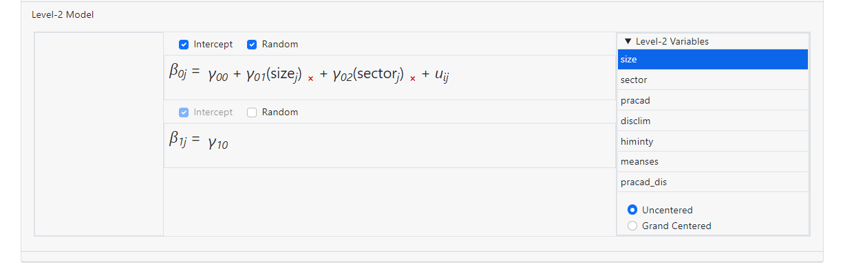 Dragging the variable SIZE on top of SECTOR as shown below
 creates a model with
a two-way interaction size*sector, but there is no longer an individual
coefficient for the variable SECTOR in the equation.
creates a model with
a two-way interaction size*sector, but there is no longer an individual
coefficient for the variable SECTOR in the equation.
How do I remove variables or change their centering
options?
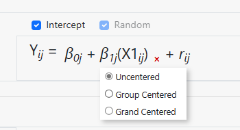
A variable may also be removed from
the model by simply clicking on the “x”
next to the variable name in the equation. The centering of a variable may also
be changed by moving the mouse over it to access the little pop-up menu below,
on which an alternative form of centering may be selected.
What graphs can I get?
Currently, the
program will provide graphs for moderation analyses only. To graphs may be
obtained, a so-called simple slopes graph and a confidence interval graph.
These will be familiar to users using the online tool at Interaction Effects in MLR, LCA, and
HLM (quantpsy.org).
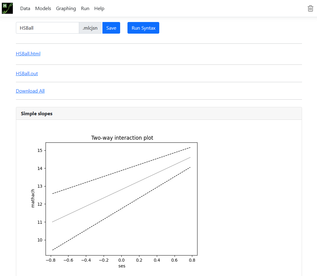
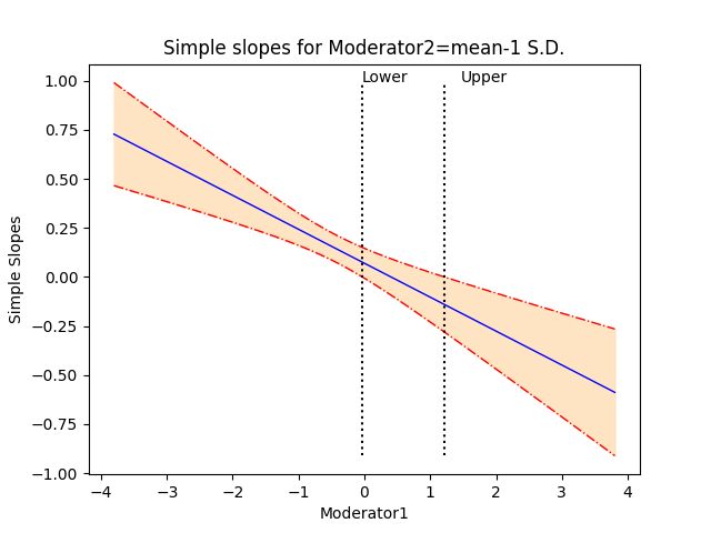
Simple slopes graph:
The first of the
available graphs is a graph of the conditional regression line(s) describing
the relationship between the outcome and the focal predictor as a function of
the moderator. The graph will automatically show a line at each of three values
of the focal variable: mean – 1 standard deviation, mean, and mean + 1
standard deviation. In other words, the value of the focal variable is held
constant at three specific values. Values of the moderating variable are used
to define the x-axis, and the graph is confined to the area (mean of moderator
– 2 standard deviations, mean of moderator + 2 standard deviations).
Here is an example of a simple slopes graph:
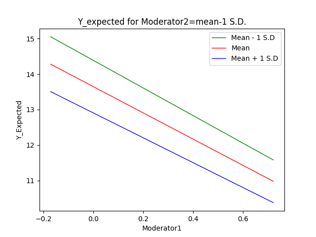 The graph is
produced as a *.png file with the name <syntax file
name>_simple_slopes.png which can easily be inserted into a paper.
A number of graph settings may also be modified by the user
on the Graphing page within the program.
Confidence interval graph:
The second graph
shows the regression line describing the relationship between the outcome and the
focal predictor as a function of the moderator, along with a 95% confidence
interval. It also shows the so-called region of significance, provided that the
boundaries of this region falls within the scale set by the values of the
moderator variable, which again defines the x-axis. The region between the
lower and upper bound of the region of significance indicates the values of the
moderator for which the slope of the regression of outcome on focal variable
transitions from non-significance to significance. The graph produced by the
program is saved to a *.png file with the name <syntax file
name>_confidence_interval.png. An example of the confidence interval
graph with regions of significance is shown below.
The graph is
produced as a *.png file with the name <syntax file
name>_simple_slopes.png which can easily be inserted into a paper.
A number of graph settings may also be modified by the user
on the Graphing page within the program.
Confidence interval graph:
The second graph
shows the regression line describing the relationship between the outcome and the
focal predictor as a function of the moderator, along with a 95% confidence
interval. It also shows the so-called region of significance, provided that the
boundaries of this region falls within the scale set by the values of the
moderator variable, which again defines the x-axis. The region between the
lower and upper bound of the region of significance indicates the values of the
moderator for which the slope of the regression of outcome on focal variable
transitions from non-significance to significance. The graph produced by the
program is saved to a *.png file with the name <syntax file
name>_confidence_interval.png. An example of the confidence interval
graph with regions of significance is shown below.
Can graphs be modified?
Graphs can be
modified using the Graphing page. This page is only available for moderation
analyses. When this page is first opened, all options are set to default
values. By default, both a simple slope and confidence interval graph using
these settings will be produced. To
request only one type of graph, simply uncheck the check box next to Simple slopes
or Confidence interval.
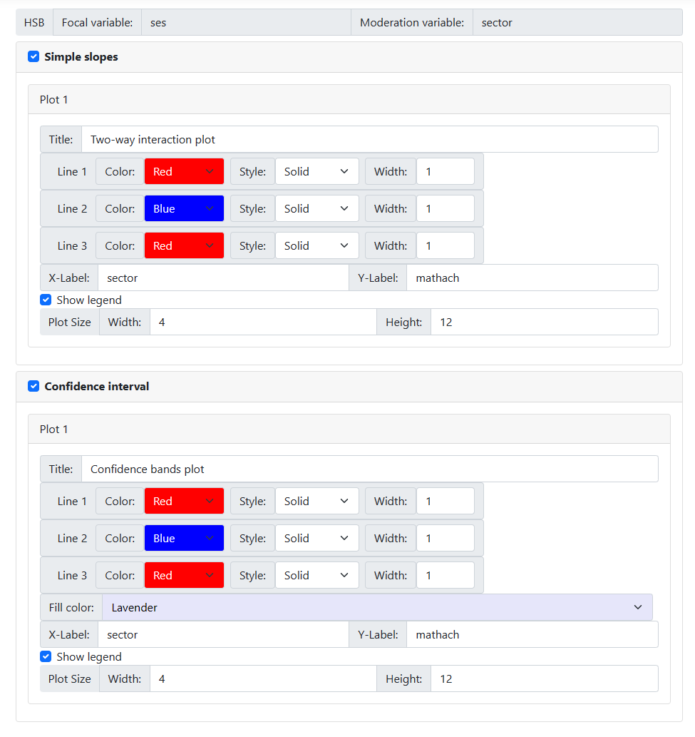 All options may be
changed. For moderation model 1, there will only be one simple slopes graph
and/or one confidence interval graph; for models 2 and 3 there will be three of
each. In all cases, however, the following options apply:
All options may be
changed. For moderation model 1, there will only be one simple slopes graph
and/or one confidence interval graph; for models 2 and 3 there will be three of
each. In all cases, however, the following options apply:
-
Title: The default title is displayed in
the Title field and may be changed according to user preferences.
-
Line color, style and width:
one of eight colors may be selected using one of four styles and in three
widths.
-
X-label and Y-label: By default,
variable names appear as axes labels. This too can be changed by the user.
-
In the case of a simple slopes graphs, the user
can show the legend (default) or opt to suppress it by unchecking the
check box next to this option.
-
The graph size may also be changed, but
readers should note that the default of a width of 4 x 12 works well for most
cases.
How do I center variables?
Centering of
variables is specified on the Models page and forms part of the variable
selection process. Once an outcome variable is specified, all potential
predictors at level-1 is accessed by clicking on the Level-1 variables
list to the right of the window.
 The user can either
enter variables into the model individually or as a group. By default,
predictors are entered uncentered. Alternatively, one can enter
variable(s) as either group centered or grand centered at lower levels of the
hierarchy, or as grand centered on the highest level of the model.
Consider the
following level-1 model for a two-level model:
The user can either
enter variables into the model individually or as a group. By default,
predictors are entered uncentered. Alternatively, one can enter
variable(s) as either group centered or grand centered at lower levels of the
hierarchy, or as grand centered on the highest level of the model.
Consider the
following level-1 model for a two-level model:
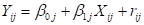 The intercept
  represents the
expected outcome for subject from level-2 unit j who has a value
of 0 on the predictor variable
represents the
expected outcome for subject from level-2 unit j who has a value
of 0 on the predictor variable  . This is the expected outcome if
is used in its
original, uncentered form.
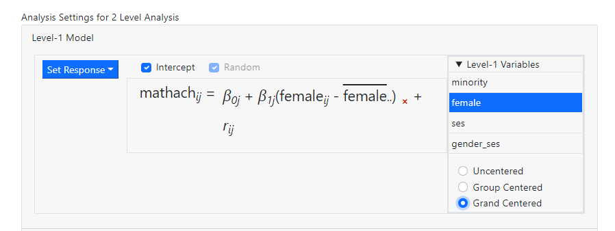
If the predictor is used as a grand
mean centered predictor, the model becomes
. This is the expected outcome if
is used in its
original, uncentered form.
If the predictor is used as a grand
mean centered predictor, the model becomes
 where
where  represents the
grand mean of all values,
irrespective of the unit the value originates from.
If the predictor is used as a group
mean centered predictor, the model becomes
represents the
grand mean of all values,
irrespective of the unit the value originates from.
If the predictor is used as a group
mean centered predictor, the model becomes
 where
where  the group mean of all
values from the j-th level-2 unit. There are as many group means as there are
level-2 units.
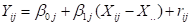
In the table below,
a small illustration of the numerical effect of group-mean and grand-mean
centering is given for 2 hypothetical level-2 units.
the group mean of all
values from the j-th level-2 unit. There are as many group means as there are
level-2 units.
In the table below,
a small illustration of the numerical effect of group-mean and grand-mean
centering is given for 2 hypothetical level-2 units.
 Note that there is a
marked difference between the raw data for the two units, yet after group-mean
centering they are the same.
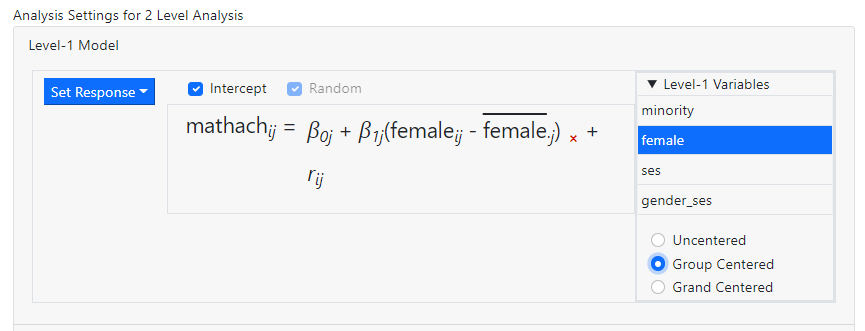
The images below
show the notation used to indicate the three options.
Note that there is a
marked difference between the raw data for the two units, yet after group-mean
centering they are the same.
The images below
show the notation used to indicate the three options.
 Multiple variables
may be selected simultaneously, and the choice of centering selected would
apply to all the selected variables. The user has the option to apply the same
three centering options to the selection made.
When multiple
variables are selected simultaneously, another option is displayed in the Level-1
Variables field, offering the option to enter the selected variables as
individual predictors or as an interaction term between the selected variables.
The entry in the level-1 model will depend on the choice between the two
options given below the list of variable names. In this case, between minority
+ ses and minority*ses.
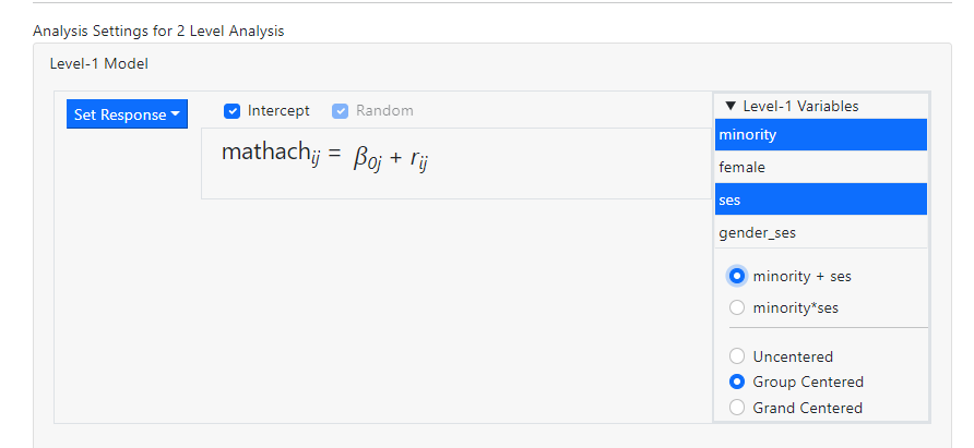
If, for example, we
want to add the predictors MINORITY and SES as individual group mean centered
variables into the level-1 equation, the following selection is made:
Multiple variables
may be selected simultaneously, and the choice of centering selected would
apply to all the selected variables. The user has the option to apply the same
three centering options to the selection made.
When multiple
variables are selected simultaneously, another option is displayed in the Level-1
Variables field, offering the option to enter the selected variables as
individual predictors or as an interaction term between the selected variables.
The entry in the level-1 model will depend on the choice between the two
options given below the list of variable names. In this case, between minority
+ ses and minority*ses.
If, for example, we
want to add the predictors MINORITY and SES as individual group mean centered
variables into the level-1 equation, the following selection is made:
 After dragging the
variables into the level-1 equation, the model becomes
After dragging the
variables into the level-1 equation, the model becomes
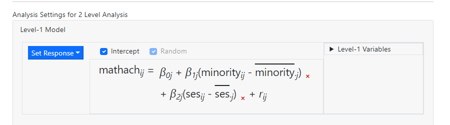 with the two
predictors added as independent, group centered predictors.
Should the
interaction term be required, the corresponding selection will look like this
with the two
predictors added as independent, group centered predictors.
Should the
interaction term be required, the corresponding selection will look like this
 and the model will
be updated to
and the model will
be updated to
 showing the inclusion of the group centered interaction
between the two variables MINORITY and SES. These images illustrate the
difference between the option minority + ses and minority*ses.
showing the inclusion of the group centered interaction
between the two variables MINORITY and SES. These images illustrate the
difference between the option minority + ses and minority*ses.
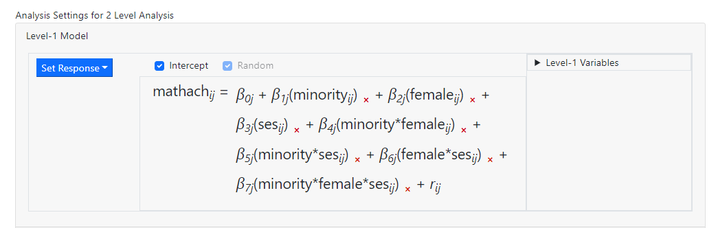
How many interactions can be included in the model?
The maximum number
of interactions allowed in the program is a 3-way interaction, in other words,
an interaction of the form a*b*c. There are no limits on the number of
individual 2-way or 3-way interactions.
In the level-1 model
below, three predictors have been entered. 2-way Interactions between all
possible pairs of the variables are also present in the model (for example minority*ses),
along with a 3-way interaction (minority*female*ses).
While it is possible to add more than 3 predictors simultaneously, selecting
more than three variables at the same time will disable the option on the Level-1
Variables box that allows for creating an interaction effect.
 Turning to
higher-levels, the type of interaction that can be added to the model depends
on the equation the selection is to be added to.
Consider the model
Turning to
higher-levels, the type of interaction that can be added to the model depends
on the equation the selection is to be added to.
Consider the model
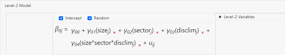
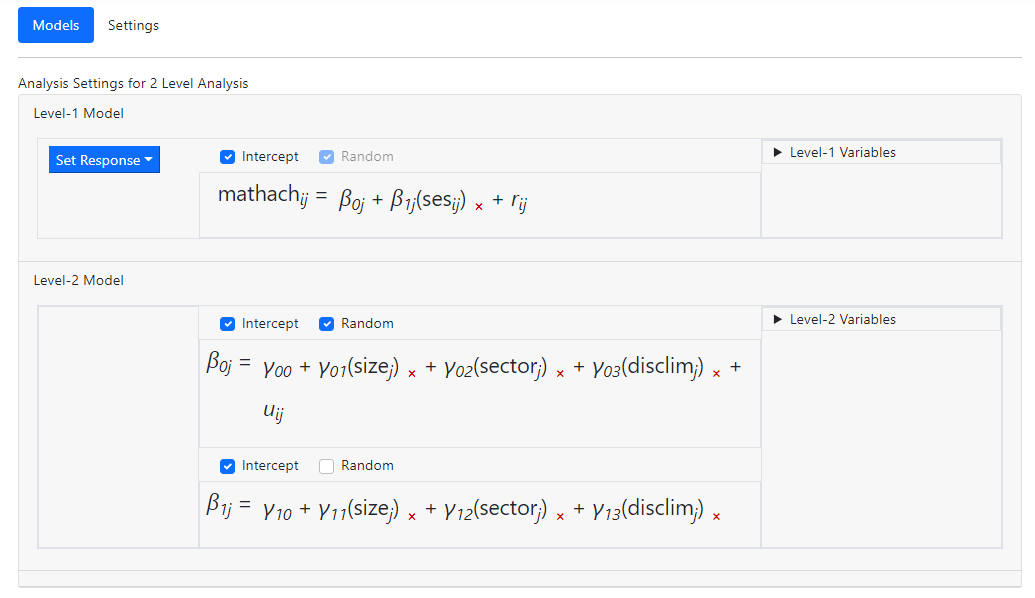 Suppose we would
like to add an interaction term to the two level-2 equations. In the case of
the first equation, that for
Suppose we would
like to add an interaction term to the two level-2 equations. In the case of
the first equation, that for  a three-way
interaction term of the form size*sector*disclim may be added
to obtain the equation
a three-way
interaction term of the form size*sector*disclim may be added
to obtain the equation
 When we attempt to
add a similar term to the second level-2 equation for
When we attempt to
add a similar term to the second level-2 equation for  ,
the program does not allow this. When we drag the interaction term into the equation, an
,
the program does not allow this. When we drag the interaction term into the equation, an  Why the difference
in behavior? The answer lies in the fact that
is the intercept equation, but
Why the difference
in behavior? The answer lies in the fact that
is the intercept equation, but  is a slope equation.
If we substitute the into the level-1
equation, we obtain
is a slope equation.
If we substitute the into the level-1
equation, we obtain
 However, if we could , we would get
 and the last term,
  , would be a four-way interaction.
Although the same level-2 variables appear on the two level-2 equations, those on the equation
for are already
multiplied with the values of the level-1 predictor SES. This implies that for
this equation, only 2-way interaction terms may be added so as not to exceed
the program limit of maximum three terms a*b*c. If we had managed to add the
three-way interaction to the second equation, we would in effect have added a
4-way interaction of the form a*b*c*d.
Apart from the 3-way
interaction limit, there is no limit on the number of individual 2- or 3-way
interaction terms that can be added to the model. In other words, a model with
10 2-way interactions and 4 3-way interactions would, theoretically be
possible, if somewhat inadvisable in terms of estimation.
, would be a four-way interaction.
Although the same level-2 variables appear on the two level-2 equations, those on the equation
for are already
multiplied with the values of the level-1 predictor SES. This implies that for
this equation, only 2-way interaction terms may be added so as not to exceed
the program limit of maximum three terms a*b*c. If we had managed to add the
three-way interaction to the second equation, we would in effect have added a
4-way interaction of the form a*b*c*d.
Apart from the 3-way
interaction limit, there is no limit on the number of individual 2- or 3-way
interaction terms that can be added to the model. In other words, a model with
10 2-way interactions and 4 3-way interactions would, theoretically be
possible, if somewhat inadvisable in terms of estimation.
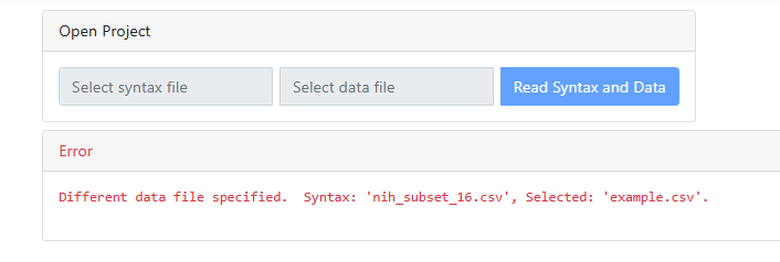
Explanation of GUI error messages
When reading in a
syntax and data file for a previous analysis, a mismatch between syntax and
data may occur, prompting the display of the message shown below. The program
will tell you what data you selected, and what you should have selected to go
with the selected syntax file.
 Should you attempt
to access the Models, Settings, Graphing or Run
page without having first completed the Data page, the program will warn
you about the omission:
Should you attempt
to access the Models, Settings, Graphing or Run
page without having first completed the Data page, the program will warn
you about the omission:
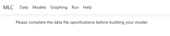 This message will
also appear if a data file has been opened, but no variable selection has been
performed and/or the Update button was not clicked upon completion of
selection.
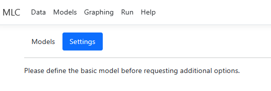
If data have been
specified, but no model has been set up via the Models page, the Settings
page will be unavailable until the Models page has been completed.
This message will
also appear if a data file has been opened, but no variable selection has been
performed and/or the Update button was not clicked upon completion of
selection.
If data have been
specified, but no model has been set up via the Models page, the Settings
page will be unavailable until the Models page has been completed.
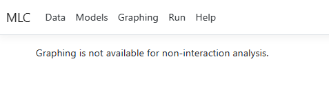
 When attempting to
access the Graphing page for a non-moderation analysis, the program will
remind you that graphing is only available for moderation analyses.
When attempting to
access the Graphing page for a non-moderation analysis, the program will
remind you that graphing is only available for moderation analyses.