FAQ: Analysis
The topics listed below address some of the questions that may arise during analysis:
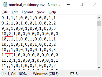
How should missing data be specified?
Missing data should not have a value in the CSV file. If the
CSV file contains any code (see, for example, the 99s in the image below)
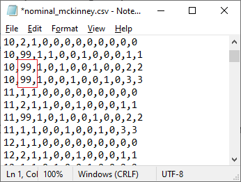 the code will be read as a valid data value, leading to incorrect
results. Instead, there should be no entry whatsoever in the case of missing
data. The CSV file should contain “,,” instead, as shown below.
the code will be read as a valid data value, leading to incorrect
results. Instead, there should be no entry whatsoever in the case of missing
data. The CSV file should contain “,,” instead, as shown below.
Which link functions are available for analysis using adaptive quadrature?
The link functions available are the log,
logistic, complimentary log-log, log-log, probit, power, and identity. Here is
a summary of link functions by distribution.
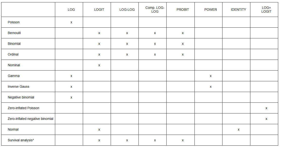 * Survival analysis, like the ordinal and nominal models, is
part of the multinomial family. In the current program, we have opted to let
the user specifically select a survival model during analysis.
* Survival analysis, like the ordinal and nominal models, is
part of the multinomial family. In the current program, we have opted to let
the user specifically select a survival model during analysis.
Which models can be used for analysis using adaptive
quadrature?
A brief description of the available options is given below.
For detailed information on these, please see our technical
information page.
Bernoulli
The Bernoulli
distribution is a discrete distribution. Variables that have a Bernoulli
distribution can take one of two values. An example of a variable with a
Bernoulli distribution is a coin toss, where the outcome is either heads
(success) or tails (failure). The probability of a success is p, where 0
< p <1.
Four link functions
are available for use with the Bernoulli distribution: logit, complimentary
log-log, probit, and log-log.
Binomial
The Binomial
distribution is a discrete distribution in which the outcome is binary. While
the Bernoulli distribution is used to describe the outcome of a single trial of
an event, the Binomial distribution
is used when the outcome of an event is observed multiple times.
Four link functions
are available for use with the Binomial distribution: logit, complimentary
log-log, probit, and log-log.
Gamma
The gamma
distribution is a two-parameter continuous probability distribution. It occurs
when the waiting times between Poisson distributed events are relevant.
Two link functions are
available for use with the Gamma distribution: log and power.
Inverse Gaussian
The inverse Gaussian distribution is a two-parameter family
of continuous probability distributions, first studied in relation to Brownian
motion. This distribution is one of a family of distributions that have been
called the Tweedie distributions, named after M.C.K. Tweedie who first used the
name Inverse Gaussian as there is an inverse relationship between the time to
cover a unit distance and distance covered in unit time.
Negative Binomial
The negative
binomial distribution is a discrete probability distribution. It is used to
model the number of successes in a sequence of independent and identically
distributed Bernoulli trials before a specified, nor random, number of failures
occurs. The negative binomial model is an extension of the Poisson model, in
the sense that it adds a normally distributed overdispersion effect.
For this model, the log link function is used.
Nominal
The nominal model
is part of a family of models based on the multinomial distribution. The
multinomial distribution is a generalization of the Binomial distribution. It
is commonly used in to describe the probability of the outcome of n independent trials each of which leads to a
success for one of c categories, with each category having a given fixed
probability of success. A nominal variable has categories that cannot be
ordered.
For the nominal model, the logistic link function is
specified.
Normal distribution (GLIM)
Generalized linear
model (GLIM) for continuous normally distributed data. This model may be used
to check on the validity of the assumption of normality for a model run with
Normal (HLM). If the assumption of normality is reasonable, results should
correspond. If not, the inverse Gaussian and Gamma distributions should be
investigated as alternative distributions for the outcome variable.
For the Normal (GLIM) model, only the identity link function
is available.
Normal distribution (HLM)
Full maximum likelihood estimation for continuous normally
distributed data. To check the validity of the assumption of normality, the
Normal (GLIM) distribution may be used.
Ordinal
The ordinal model
is also part of a family of models based on the multinomial distribution. The
multinomial distribution is a generalization of the Binomial distribution. It
is commonly used in to describe the probability of the outcome of n independent trials each of which leads to a
success for one of c categories, with each category having a given fixed
probability of success. An ordinal outcome is an outcome whose levels can be
ordered.
For the ordinal model four link functions are available:
cumulative logit link, cumulative complimentary log-log link, cumulative
probit, and cumulative log-log link.
Poisson
The Poisson
distribution is a discrete frequency distribution that gives the probability of
several independent events occurring in a fixed time, given the average number
of times the event occurs over that time period.
For the Poisson distribution, the model is transformed to a
linear model by using the log link function.
Survival analysis
The survival analysis
model is used to describe the expected duration of time until one or more
events occur. Observations are censored, in that for some units the event of
interest did not occur during the entire time period studied. In addition,
there may be predictors whose effects on the waiting time need to be controlled
or assessed.
The following link functions are available: complimentary
log-log (proportional hazards), logit, probit, and log-log link.
Zero-inflated Poisson
The zero-inflated
Poisson model is a mixture model used to model count data that has an excess of
zero counts. It is assumed that for non-zero counts the counts are generated
according to a Poisson model.
This model is estimated using a log link function for the
Poisson component (modelling non-zero responses), and a logit link function for
the zero-inflated component (modeling the zero response)
Zero-inflated negative binomial
The zero-inflated negative Binomial model is a mixture
model used to model count data that has an excess of zero counts. It is assumed
that the count in the not-always-zero group has a negative binomial
distribution.
This model is estimated using a log link function for the
negative binomial component (modelling non-zero responses), and a logit link
function for the zero-inflated component (modeling the zero response)
What methods of estimation are used?
Models with normally distributed outcomes are estimated by
full Maximum Likelihood. For starting values, the solution obtained when all
random effects are set to identity is used.
For models with binary, ordinal, count, and nominal
outcomes, or when a normal distribution with an identity link function is
specified, two methods of estimation are available: maximization of the
posterior distribution (MAP) and numerical integration (adaptive and non-adaptive
quadrature) to obtain parameter and standard error estimates.
The MAP method of estimation can be used to
obtain a point estimate of an unobserved quantity based on empirical data. It
is closely related to Fisher's method of maximum likelihood but
employs an augmented optimization objective which incorporates a prior
distribution over the quantity one wants to estimate.
Adaptive quadrature estimation is a numeric method for
evaluating multi-dimensional integrals. For mixed effect models with count and
categorical outcomes, the log-likelihood function is expressed as the sum of
the logarithm of integrals, where the summation is over higher-level units, and
the dimensionality of the integrals equals the number of random effects.
Typically, MAP estimates are used as starting values for the quadrature procedure. When the
number of random effects is large, the quadrature procedures can become
computationally intensive. In such cases, MAP estimation is usually selected as the
final method of estimation.
Numerical quadrature, as implemented here, offers users a
choice between adaptive and non-adaptive quadrature. Quadrature uses a
quadrature rule, i.e., an approximation of the definite integral of a function,
usually stated as a weighted sum of function values at specified points within
the domain of integration. Adaptive quadrature generally requires fewer points
and weights to yield estimates of the model parameters and standard errors that
are as accurate as would be obtained with more points and weights in
non-adaptive quadrature. The reason for that is that the adaptive quadrature
procedure uses the empirical Bayes means and covariances, updated at each
iteration to essentially shift and scale the quadrature locations of each
higher-level unit to place them under the peak of the corresponding integral.
The algorithm used is based on the maximization of the posterior distribution (MAP) with respect to the random
effects.
What is the difference between unit specific and
population average results?
The regression parameters in multilevel generalized linear
models have the “unit specific” or conditional interpretation, in
contrast to the “population averaged” or marginal estimates that
represent the unconditional covariate effects. HLMix
uses numerical quadrature to obtain population average estimates from their
unit specific counterparts in models with multiple random effects. Standard
errors for the population average estimates are derived using the delta method.
In addition to the “unit specific” estimates, the population
average estimates are also provided as part of the output file.
For more on this topic, please see:
Hedeker, Donald; du Toit, Stephen
H. C.; Demirtas, Hakan; Gibbons, Robert D. (2018). Note on
marginalization of regression parameters from mixed models of binary outcomes [2018], Biometrika, 74, 354-361.
https://www.stata.com/support/faqs/statistics/random-effects-versus-population-averaged/
Should I use Normal (HLM) or Normal(GLIM) for a
continuous normally distributed outcome?
Both these distributions may be used. The purpose of the
Normal (GLIM) option is to check on the validity of the assumption of normality
for a model run with Normal (HLM). If the assumption of normality is
reasonable, results should correspond. If not, the inverse Gaussian and Gamma
distributions should be investigated as alternative distributions for the
outcome variable.
How should weights be specified?
If a level-1
weight is to be specified, this should be done next by checking the check box
in the Weight1 field under the weighting variable’s column on the Data
page. Selection of additional weights at higher levels for HLM models are done
in the same way. For a GLIM model, only the Weight1 field should be
used.