Nominal-logit model for
McKinney data
In this example we use data from the McKinney Homeless ResearchProject study (Hough, et. al.,
1997; Hurlburt, et. al. 1996) to illustrate the fitting of a nominal
model. For information on specific topics, please use the links below:
The data
The
McKinney Homeless Research Project study was
designed to evaluate the effectiveness of using Section 8 certificates to
provide independent housing to the severely mentally ill homeless. These
housing certificates, which require clients to pay 30% of their income toward
rent, are meant to enable low-income subjects to choose and obtain independent
housing in the community. Three hundred sixty-two clients took part in this
longitudinal study employing a randomized factorial design. Clients were
randomly assigned to one of two types of case management (comprehensive vs.
traditional) and to one of two levels of access to independent housing (using
Section 8 certificates). The project was restricted to clients diagnosed with a
severe and persistent mental illness who were either homeless or at high risk of becoming homeless
at the start of the study. Individuals' housing status was classified at
baseline and at 6-, 12-, and 24-month follow-ups. Here, we focus on examining
the effect of access to Section 8 certificates on housing outcomes across time.
At each time point, subjects' housing status was classified as either
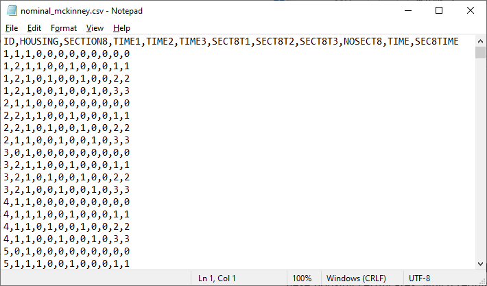
streets/shelters, community housing, or independent housing; a partial list of
these data is given below in the form of a comma separated values (CSV) file, named
nominal_mckinney.csv.
-
ID is the subject ID (362 subjects in total).
-
HOUSING represents the housing status at
the time of interview: 0 = street, 1 = community, 2 = independent.
-
SECTION8 indicates the Section 8 group,
with 1 representing those using Section 8 certifications, and 0 those without.
-
TIME1 to TIME3 are three dummy variables for time
effects, and denote whether a classification was at baseline, or at the 6-, 12-
or 24-month follow-up. If at the 6 months follow-up, TIME1 = 1 and TIME2 = TIME3 =0;
if at 12 months, TIME2 = 1 while TIME1 = TIME3 = 0; and at the 24-month
follow-up TIME3 = 1 and TIME1 = TIME2 = 0. With this coding scheme, the baseline serves as the reference
group of classification. The coding structure is shown in the table below.
-
Three Section 8 by time interaction terms follow: SECT8T1 is the product of SECTION8 and TIME1, and SECT8T2
and SECTION8 the products of SECTION8 and TIME2 and TIME3 respectively.
-
NOSECT8 indicates the non-Section 8 group, with 0 = no, and 1 = yes.
-
TIME represents the linear time contrast. At baseline, TIME = 0,
at 6 months, TIME = 1, at 12 months TIME = 2, and at 24 months TIME = 3.
-
SEC8TIME is the product of SECTION8 and TIME.
Coding of the dummy variables TIME1, TIME2, and TIME3
| TIME1 | TIME2 | TIME3 | TIME
| baseline | 0 | 0 | 0 | 0 |
| 6 months | 1 | 0 | 0 | 1 |
| 12 months | 0 | 1 | 0 | 2 |
| 24 months | 0 | 0 | 1 | 3 |
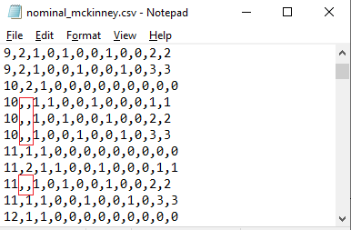
There are missing data for the housing
status variable. Thus, some subjects are measured at all four time points and
others at fewer time points. Data from these time points with missing values
are not used in the analysis; however, data are used from other time points
where there are no missing data. Thus, for inclusion into the analysis, a
subject's data (both the dependent variable and all explanatory variables used
in a particular analysis) at a specific time point must be complete. The number
of repeated observations per subject depends on the number of time points for
which there are non-missing data for that subject. The correct way to specify
missing data is to enter no value into the CSV file.
The CSV file should contain “,,” instead, as shown below.
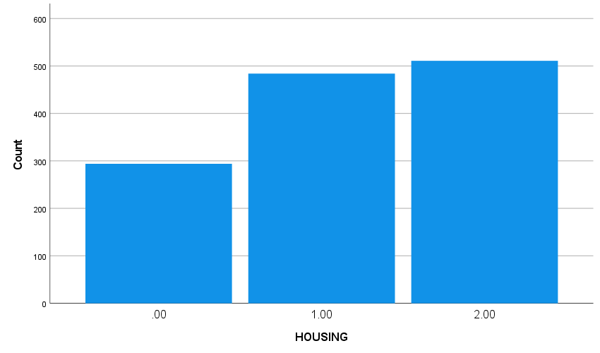
 A bar chart of the variable HOUSING is given below. Housing status at
the beginning of the study was mostly independent or in community housing. As
we would like to compare these categories to the “street” category,
we will be using the first category of HOUSING as reference category in the
analysis to follow.
A bar chart of the variable HOUSING is given below. Housing status at
the beginning of the study was mostly independent or in community housing. As
we would like to compare these categories to the “street” category,
we will be using the first category of HOUSING as reference category in the
analysis to follow.
 The observed sample sizes and response proportions by group are given in the table
below. These observed proportions indicate a general decrease in street living
and an increase in independent living across time for both groups. The increase
in independent housing, however, appears to occur sooner for the section 8
group relative to the control group. Regarding community living, across time
there is an increase for the control group and a decrease for the section 8
group.
Regarding missing data, further inspection of indicates that there is some attrition
across time; attrition rates of 19.4% and 12.7% are observed at the final time
point for the control and section 8 groups, respectively. In addition, one
subject provided no housing data at any of the four measurement time points.
Since estimation of model parameters is based on a full-likelihood approach,
missing data are assumed to be "ignorable" conditional on both the
explanatory variables and observed nominal responses (Laird, 1988). In
longitudinal studies, ignorable nonresponse falls under Rubin's (1976)
"missing at random" (MAR) assumption, in which the missingness
depends only on observed data. In what follows, since the focus is on
describing use of the nominal model, we will make the MAR assumption (e.g., a
mixed-effects pattern-mixture model as described in Hedeker & Gibbons
(1997)) could be used.
Observed sample sizes and response proportions by group
The observed sample sizes and response proportions by group are given in the table
below. These observed proportions indicate a general decrease in street living
and an increase in independent living across time for both groups. The increase
in independent housing, however, appears to occur sooner for the section 8
group relative to the control group. Regarding community living, across time
there is an increase for the control group and a decrease for the section 8
group.
Regarding missing data, further inspection of indicates that there is some attrition
across time; attrition rates of 19.4% and 12.7% are observed at the final time
point for the control and section 8 groups, respectively. In addition, one
subject provided no housing data at any of the four measurement time points.
Since estimation of model parameters is based on a full-likelihood approach,
missing data are assumed to be "ignorable" conditional on both the
explanatory variables and observed nominal responses (Laird, 1988). In
longitudinal studies, ignorable nonresponse falls under Rubin's (1976)
"missing at random" (MAR) assumption, in which the missingness
depends only on observed data. In what follows, since the focus is on
describing use of the nominal model, we will make the MAR assumption (e.g., a
mixed-effects pattern-mixture model as described in Hedeker & Gibbons
(1997)) could be used.
Observed sample sizes and response proportions by group
| Time point |
| Group | Status | Baseline | 6 months | 12 months | 24 months |
| Control | Street | 0.555 | 0.186 | 0.089 | 0.124 |
| Community | 0.339 | 0.578 | 0.582 | 0.455 |
| Independent | 0.106 | 0.236 | 0.329 | 0.421 |
| n | 180 | 161 | 146 | 145 |
| Section 8 | Street | 0.442 | 0.093 | 0.121 | 0.120 |
| Community | 0.414 | 0.280 | 0.146 | 0.228 |
| Independent | 0.144 | 0.627 | 0.732 | 0.652 |
| n | 181 | 161 | 157 | 158 |
In preparation for the subsequent analyses, the marginal response proportions can be converted to
the two logits of the nominal regression model (i.e., 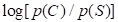 and
and 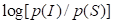 ,
where S = street, C = community, and I = independent housing).
These logits are given below.
Logits across time by group
,
where S = street, C = community, and I = independent housing).
These logits are given below.
Logits across time by group
| Time point |
| Group | Status | Baseline | 6 months | 12 months | 24 months |
| Control | Community vs. Street | -0.49 | 1.13 | 1.88 | 0.130 |
| Independent vs. Street | -1.66 | 0.24 | 1.31 | 1.22 |
| Time point |
| Section 8 | Status | Baseline | 6 months | 12 months | 24 months |
| Control | Community vs. Street | -0.07 | 1.10 | 0.19 | 0.64 |
| Independent vs. Street | -1.12 | 1.91 | 1.0 | 1.69 |
| Difference | Status | Baseline | 6 months | 12 months | 24 months |
| Control | Community vs. Street | 0.42 | -0.03 | -1.69 | -0.66 |
| Independent vs. Street | 0.54 | 1.67 | 0.49 | 0.47 |
The logits clearly show the increase in community and independent housing, relative
to street housing, at all follow-up time points (6, 12, and 24 months). In terms
of group-related differences, these appear most pronounced at 6 months for
independent housing and 12 months for community housing. While examination of
these logits is instructive, the subsequent analyses will more rigorously
assess the degree to which these logits vary by time and group.
In this example, one random subject effect (i.e., a random subject
intercept) is assumed and the repeated housing status classifications is
modeled in terms of the dummy-coded time effects (6, 12,
and 24 month follow-ups compared to baseline), a group effect (section 8 versus
control), and group by time interaction terms.
The model
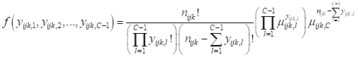
The nominal model is part of a family of models based on the
multinomial distribution, which is a generalization of the Binomial
distribution. It is commonly used in to describe the probability of the outcome
of n independent trials each of which leads to
a success for one of c categories, with each category having a given
fixed probability of success. A nominal variable has categories that cannot be
ordered.
 where C represents the number of categories of the
outcome variable.
For the nominal model, the logistic link function is
specified.
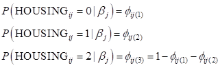
In the current example, the outcome variable HOUSING
is coded 0, 1, and 2. Therefore
where C represents the number of categories of the
outcome variable.
For the nominal model, the logistic link function is
specified.
In the current example, the outcome variable HOUSING
is coded 0, 1, and 2. Therefore
 As we wish to use the “street” category as
reference category, we select the first category as reference category and will
thus be considering the two logits
As we wish to use the “street” category as
reference category, we select the first category as reference category and will
thus be considering the two logits
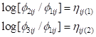 For c = 2 (community housing)
 and for c = 3
 .
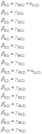
The level-2 model is
.
The level-2 model is
Reading in the data
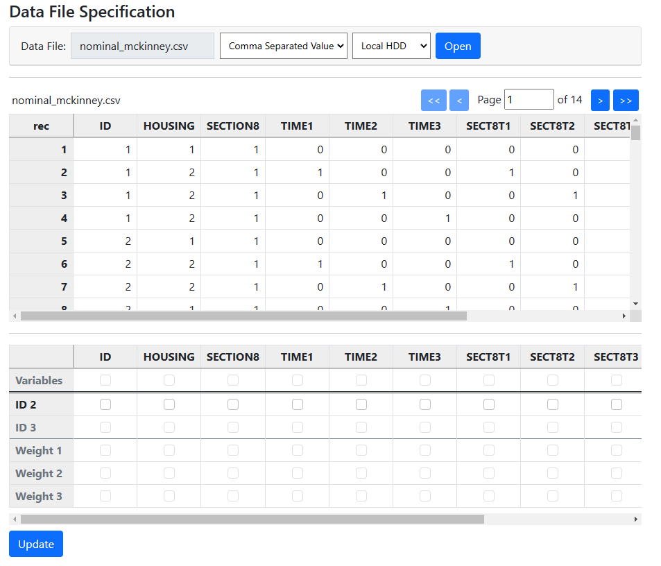
To construct this model, we select New Analysis on the landing page.
 thereby opening the Data page. Select the CSV file and click Open to
obtain the page below.
thereby opening the Data page. Select the CSV file and click Open to
obtain the page below.
 The first step is to select an ID variable. In this case, the variable ID defines
the hierarchical structure, and we select it by checking the box associated
with this variable in the ID 2 line. To select predictors, the boxes in
the Variables line must be checked. We opt to select them all
The first step is to select an ID variable. In this case, the variable ID defines
the hierarchical structure, and we select it by checking the box associated
with this variable in the ID 2 line. To select predictors, the boxes in
the Variables line must be checked. We opt to select them all
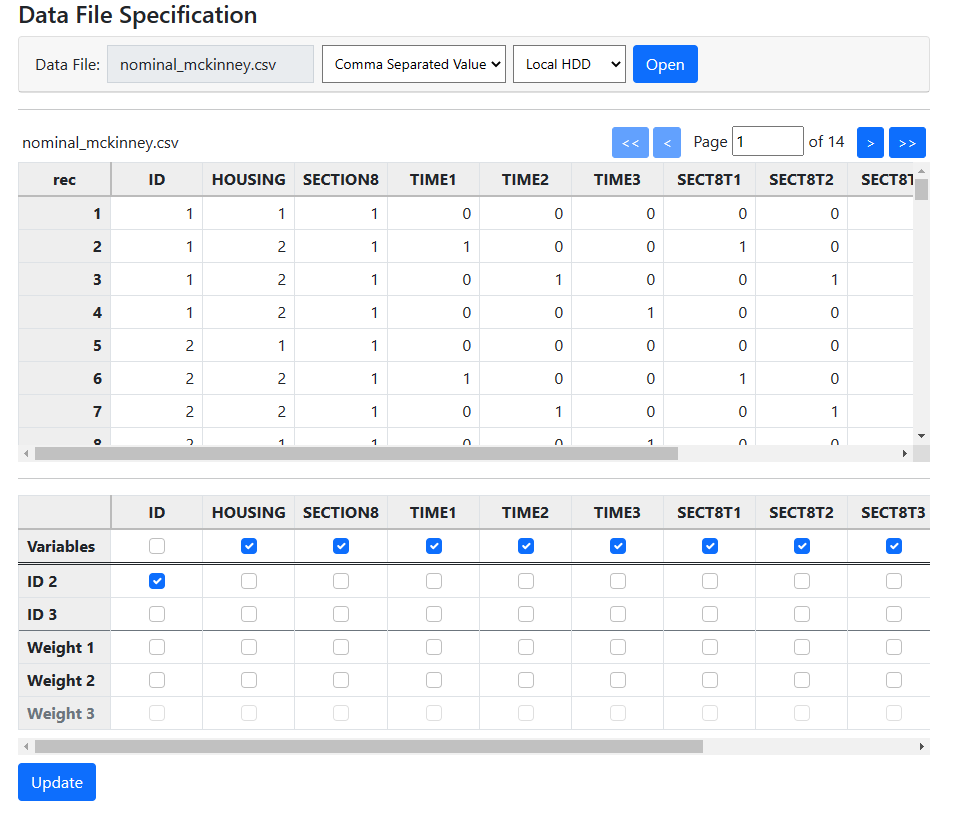 before clicking Update. Once Update is clicked the program automatically
determines the appropriate levels of all selected variables.
before clicking Update. Once Update is clicked the program automatically
determines the appropriate levels of all selected variables.
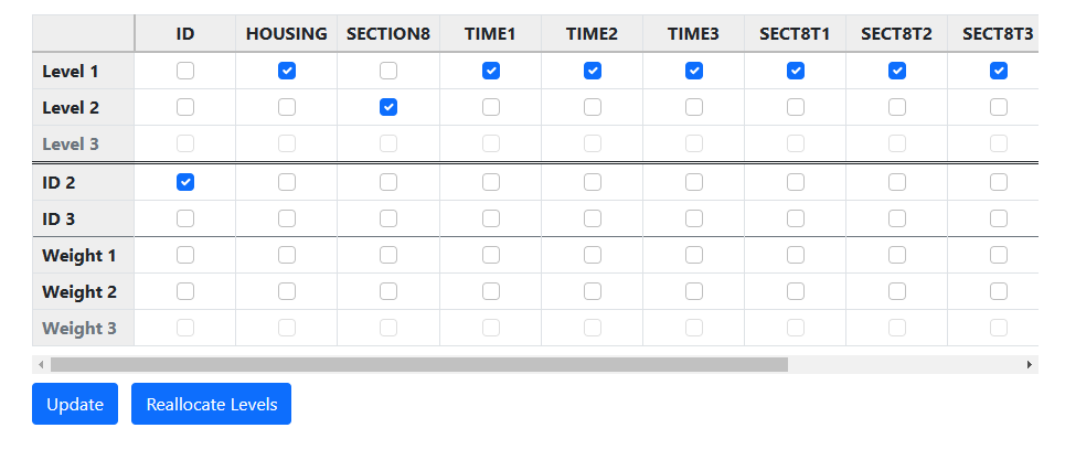 With data specification now complete, model building can begin. Click on Models
at the top of the page to move to the Models page.
With data specification now complete, model building can begin. Click on Models
at the top of the page to move to the Models page.
Building the model
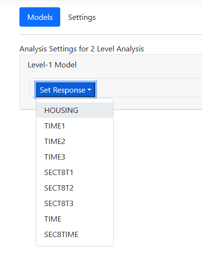
The first step is specifying the response variable. Select HOUSING from the
drop-down list associated with the Set Response field. An unconditional
model is now displayed.
 The TIME variables are selected from the Level-1 Variables field by holding
down the Control button while clicking on the names. Next, drag them all
into the level-1 equation before releasing the mouse button. The following
level-1 model appears:
The TIME variables are selected from the Level-1 Variables field by holding
down the Control button while clicking on the names. Next, drag them all
into the level-1 equation before releasing the mouse button. The following
level-1 model appears:
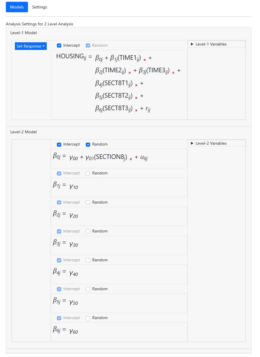
 Add the three SECTION8 variables (SECT8T1, SECT8T2 and SECT8T3) in the same way to
the level-1 equation. Then add the variable SECTION8 to the intercept equation
at level-2 to obtain the final model
Add the three SECTION8 variables (SECT8T1, SECT8T2 and SECT8T3) in the same way to
the level-1 equation. Then add the variable SECTION8 to the intercept equation
at level-2 to obtain the final model
Specification
of outcome type and associated options
Move to the Settings page by clicking on Settings at the top of the
page. When the page opens, we see that the programs has correctly suggested a
nominal model as appropriate for these data. The default values of reference
category and link function for the nominal distribution are displayed.
 As these settings are exactly what we intend to use, we need not make additional
changes here. We can proceed to run the analysis.
As these settings are exactly what we intend to use, we need not make additional
changes here. We can proceed to run the analysis.
Running the model
Run the model by going to the Run page by clicking on the Run link at
the top of the page. The Run page opens, and two options are available:
 One can Save the model information to a syntax file with file extension
MLCJSN for potential reuse. By default, the default file name assigned
corresponds to the file name of the data file. Using this option is optional,
however, and one can simply click the Run Syntax option to start the
analysis.
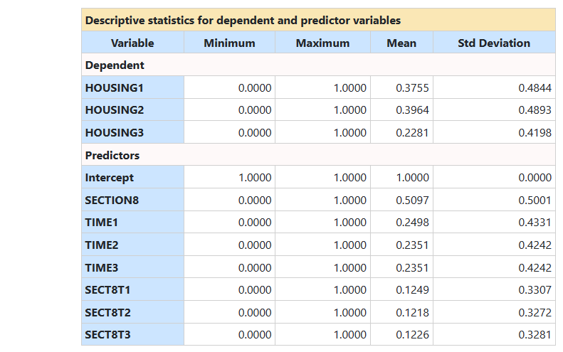
Portions of the output file are shown below. The first
part of the output file gives a description of the model specifications. This is followed by
descriptive statistics for all the variables included in the model. We note that the
most frequent response was in category 2, i.e. "Independent"
on the nominal outcome HOUSING, while 23% indicated
that they were living on the street (HOUSING = 0, the reference category here
represented by the indicator variable HOUSING3). The variable HOUSING1 represents the
respondents living in community housing.
Note that the order of the indicator variables for HOUSING is the opposite of the original coding of the variable: as we selected the
first category as reference category, the program automatically recodes it to
make the selected reference category the last category in the working data set.
One can Save the model information to a syntax file with file extension
MLCJSN for potential reuse. By default, the default file name assigned
corresponds to the file name of the data file. Using this option is optional,
however, and one can simply click the Run Syntax option to start the
analysis.
Portions of the output file are shown below. The first
part of the output file gives a description of the model specifications. This is followed by
descriptive statistics for all the variables included in the model. We note that the
most frequent response was in category 2, i.e. "Independent"
on the nominal outcome HOUSING, while 23% indicated
that they were living on the street (HOUSING = 0, the reference category here
represented by the indicator variable HOUSING3). The variable HOUSING1 represents the
respondents living in community housing.
Note that the order of the indicator variables for HOUSING is the opposite of the original coding of the variable: as we selected the
first category as reference category, the program automatically recodes it to
make the selected reference category the last category in the working data set.
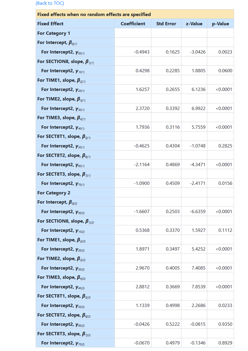
 Results for the model without any random effects are
given next. The first eight values are those for the intercept, SECTION8, TIME1,
…, SECT8T3 for response code 1 vs. code 0, the last eight are for the same predictors, but
for response code 2 vs. response code 0.
Results for the model without any random effects are
given next. The first eight values are those for the intercept, SECTION8, TIME1,
…, SECT8T3 for response code 1 vs. code 0, the last eight are for the same predictors, but
for response code 2 vs. response code 0.

 The results obtained with adaptive quadrature estimation are given next.
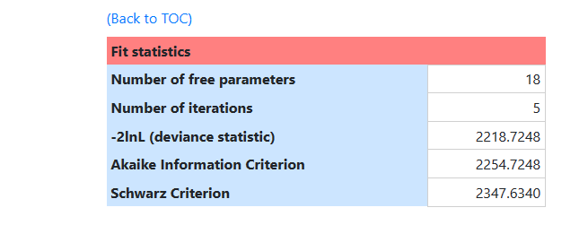 Comparing the log-likelihood value from this analysis to one where there are
no random effects clearly supports inclusion of the random subject effect
(likelihood ratio
Comparing the log-likelihood value from this analysis to one where there are
no random effects clearly supports inclusion of the random subject effect
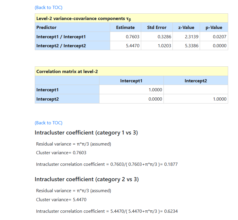
(likelihood ratio  ). Expressed as intraclass correlations
 and
and  for community versus street and independent versus street, respectively. Thus, the subject
influence is much more pronounced in terms of distinguishing independent versus
street living, relative to community versus street living. This is borne out by
contrasting models with separate versus a common random-effect variance across
the two category contrasts (not shown) which yields a highly significant
likelihood ratio
for community versus street and independent versus street, respectively. Thus, the subject
influence is much more pronounced in terms of distinguishing independent versus
street living, relative to community versus street living. This is borne out by
contrasting models with separate versus a common random-effect variance across
the two category contrasts (not shown) which yields a highly significant
likelihood ratio  favoring the
model with separate variance terms.
The unit specific results follow.
favoring the
model with separate variance terms.
The unit specific results follow.
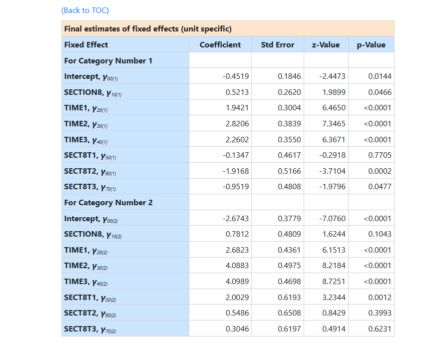 In terms of significance of the fixed effects, the time effects
are observed to be highly significant. With the inclusion of the Time by
Section 8 interaction terms, the time effects reflect
comparisons between time points for the control group (i.e., SECTION8
coded as 0). Thus, subjects in the control group show increased use of both
independent and community housing relative to street housing at all three
follow-ups, as compared to baseline. Similarly, due to the inclusion of the
interaction terms, the Section 8 effect is the group difference at baseline (i.e.,
when all time effects are 0). Using a .05 cutoff, there is no statistical
evidence of group differences at baseline. Turning to the interaction terms,
these indicate how the two groups differ in terms of comparisons between time
points. Compared to controls, the increase in community versus street housing
is less pronounced for section 8 subjects at 12 months (the estimate for
SECT8T2 equals –1.92 in terms of the logit), but not statistically
different at 6 months (SECT8T1) and only marginally
different at 24 months (SECT8T3). Conversely, as compared to controls, the increase in independent versus street
housing (response code 2 vs. code 0) is more pronounced for section 8 subjects at
6 months (the estimate equals 2.00 in terms of the logit), but not
statistically different at 12 or 24 months.
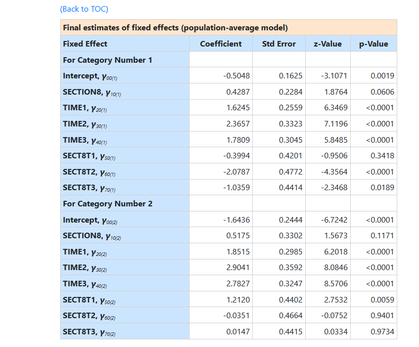
In terms of community versus street housing (i.e.,
response code 1 versus 0), there is an increase across time for the control
group relative to the Section 8 group. As the statistical test indicated, these
groups differ most at 12 months. For the independent versus street housing
comparison (i.e., response code 2 versus 0) there is a beneficial effect
of Section 8 certificates at 6 months. Thereafter, the non-significant
interaction terms indicate that the control group
catches up to some degree. Considering these results of the mixed-effects
analysis, it is seen that both groups reduce the degree of street housing but
do so in somewhat different ways. The control group subjects are shifted more
towards community housing, whereas Section 8 subjects are more quickly shifted
towards independent housing.
This differential effect of Section 8 certificates over time
is completely missed if one simply analyzes the outcome variable as a binary
indicator of street versus non-street housing (i.e., collapsing
community and independent housing categories). In this case (not shown), none
of the section 8 by time interaction terms are observed to be statistically
significant. Thus, analysis of the three-category nominal outcome is important in uncovering the beneficial
effect of Section 8 certificates.
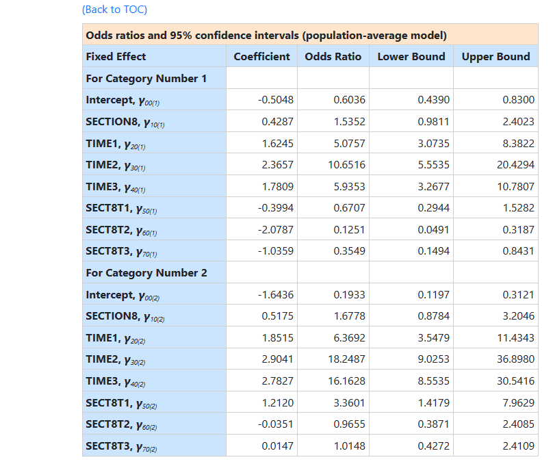
The output also includes the intracluster correlation coefficient for both categories, and population average results, as shown
below.
In terms of significance of the fixed effects, the time effects
are observed to be highly significant. With the inclusion of the Time by
Section 8 interaction terms, the time effects reflect
comparisons between time points for the control group (i.e., SECTION8
coded as 0). Thus, subjects in the control group show increased use of both
independent and community housing relative to street housing at all three
follow-ups, as compared to baseline. Similarly, due to the inclusion of the
interaction terms, the Section 8 effect is the group difference at baseline (i.e.,
when all time effects are 0). Using a .05 cutoff, there is no statistical
evidence of group differences at baseline. Turning to the interaction terms,
these indicate how the two groups differ in terms of comparisons between time
points. Compared to controls, the increase in community versus street housing
is less pronounced for section 8 subjects at 12 months (the estimate for
SECT8T2 equals –1.92 in terms of the logit), but not statistically
different at 6 months (SECT8T1) and only marginally
different at 24 months (SECT8T3). Conversely, as compared to controls, the increase in independent versus street
housing (response code 2 vs. code 0) is more pronounced for section 8 subjects at
6 months (the estimate equals 2.00 in terms of the logit), but not
statistically different at 12 or 24 months.
In terms of community versus street housing (i.e.,
response code 1 versus 0), there is an increase across time for the control
group relative to the Section 8 group. As the statistical test indicated, these
groups differ most at 12 months. For the independent versus street housing
comparison (i.e., response code 2 versus 0) there is a beneficial effect
of Section 8 certificates at 6 months. Thereafter, the non-significant
interaction terms indicate that the control group
catches up to some degree. Considering these results of the mixed-effects
analysis, it is seen that both groups reduce the degree of street housing but
do so in somewhat different ways. The control group subjects are shifted more
towards community housing, whereas Section 8 subjects are more quickly shifted
towards independent housing.
This differential effect of Section 8 certificates over time
is completely missed if one simply analyzes the outcome variable as a binary
indicator of street versus non-street housing (i.e., collapsing
community and independent housing categories). In this case (not shown), none
of the section 8 by time interaction terms are observed to be statistically
significant. Thus, analysis of the three-category nominal outcome is important in uncovering the beneficial
effect of Section 8 certificates.
The output also includes the intracluster correlation coefficient for both categories, and population average results, as shown
below.
References
Hedeker, D. & Gibbons, R.D. (2006). Longitudinal Data
Analysis. Wiley: New York.
Hedeker, D. & Gibbons, R.D. (1997). Application of random-effects pattern-mixture
models for missing data in longitudinal studies. Psychological Methods, 2(1):
64 – 78.
Hough, R.L., Harmon, S., Tarke, H., Yamashiro, S., Quinlivan,
R., Landau-Cox, P., Hurlburt, M.S., Wood, P.A., Milone, R., Renker, V.,
Crowell, A. & Morris, E., (1997). Supported independent housing:
Implementation issues and solutions in the San Diego McKinney Homeless
Demonstration Research Project. In W.R. Breakey & J.W. Thompson (eds.), Mentally
Ill and Homeless: Special Programs for Special Needs, pp. 95-117. New York:
Harwood Academic Publishers.
Hurlburt, M.S., Wood, P.A., & Hough, R.L. (1996).
Providing independent housing for the homeless mentally ill: a novel approach
to evaluating long-term longitudinal housing patterns, Journal of Community
Psychology, 24, 291-310.