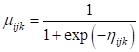
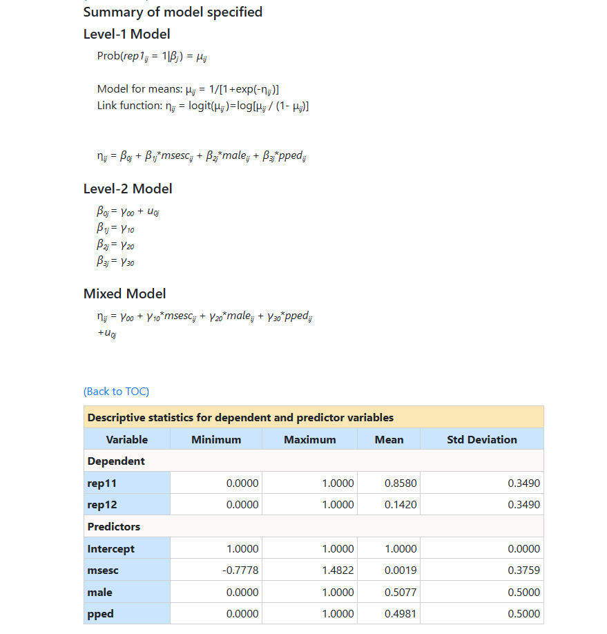
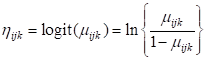
Bernoulli model with logit link function
The data
Data are from a national survey of primary education in Thailand conducted in 1988, and yielding, for our analysis, complete data on 7516 sixth graders nested within 356 primary schools. Of interest is the probability that a child will repeat a grade during the primary years. The first few lines of the comma separated values (CSV) file thai_all_u.csv are shown below.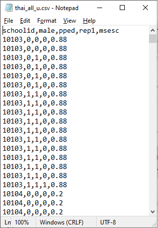 Inspection of the outcome variable REP1 shows that 86% of the
students did not repeat a grade, and 14% did. Roughly half of students had
pre-primary education. The mean SES of schools ranged between -0.77 and
1.49, with mean approximately equal to zero.
Inspection of the outcome variable REP1 shows that 86% of the
students did not repeat a grade, and 14% did. Roughly half of students had
pre-primary education. The mean SES of schools ranged between -0.77 and
1.49, with mean approximately equal to zero.
The model
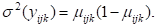
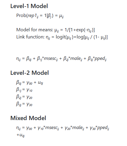
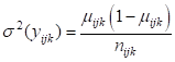
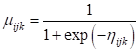
It is hypothesized that the child’s gender, pre-primary experience and the school mean SES will be associated with the probability of repetition. Every level-1 record corresponds to a student, with a single binary outcome per student, so the model type is Bernoulli. The sampling distribution of the Bernoulli distribution is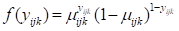 and the variance is
 Inspection of the outcome variable shows that 86% of the
students did not repeat a grade, and 14% did. Roughly half of students had
pre-primary education. The mean of schools ranged between -0.77 and 1.49, with mean approximately equal to
zero.
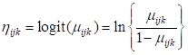
Using the logit link function, the model we consider is:
Inspection of the outcome variable shows that 86% of the
students did not repeat a grade, and 14% did. Roughly half of students had
pre-primary education. The mean of schools ranged between -0.77 and 1.49, with mean approximately equal to
zero.
Using the logit link function, the model we consider is:
 The model for the means can be expressed as
 The model we intend to fit can be formulated as
Reading in the data
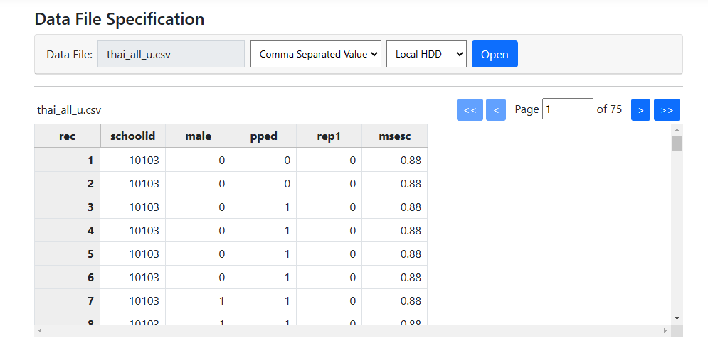
To start a new analysis, select the New Analysis option on the landing page. The Data page will open. As a first step, select the
data file thai_all_u.csv and click Open to obtain the image shown
below. Note that the data file may reside on a local hard drive, OneDrive, or
Google Drive. A description of the variables contained in the data file are
given below the image.
The Data page will open. As a first step, select the
data file thai_all_u.csv and click Open to obtain the image shown
below. Note that the data file may reside on a local hard drive, OneDrive, or
Google Drive. A description of the variables contained in the data file are
given below the image.
 The following information is available:
- REP1 indicates whether a child repeated a grade (1 if yes, 0 if no).
- MALE = 1 if the student is male and 0 if female.
- If a student had pre-primary experience, PPED = 1. For students without pre-primary experience , PPED= 0.
- At the school level, the school mean socio-economic status is represented by the variable
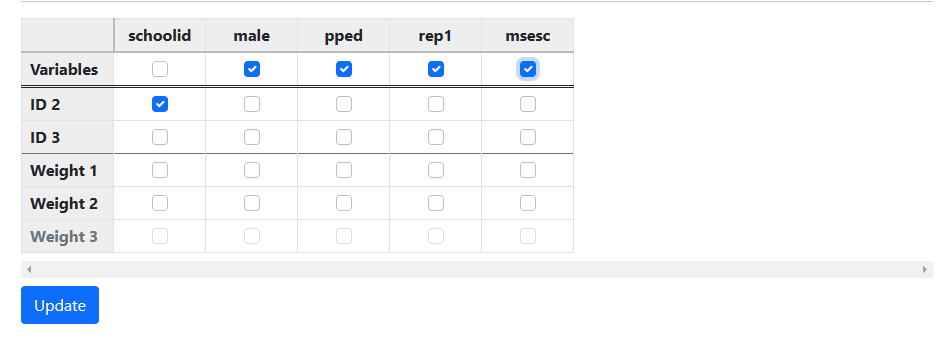 Finally, we click update to
prompt the program to automatically allocate the variables at the appropriate
levels. When complete, the page updates to
Finally, we click update to
prompt the program to automatically allocate the variables at the appropriate
levels. When complete, the page updates to
 Data file specification complete, we can now move to model
building. Click on Models on the main menu bar to move on to the Models
page.
Data file specification complete, we can now move to model
building. Click on Models on the main menu bar to move on to the Models
page.
Model building
Model building starts with selection of the outcome variable using the Set Response field. In this case, the outcome variable is REP1. Select the variable as shown below.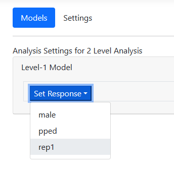 The page automatically updates to display an unconditional
model.
The page automatically updates to display an unconditional
model.
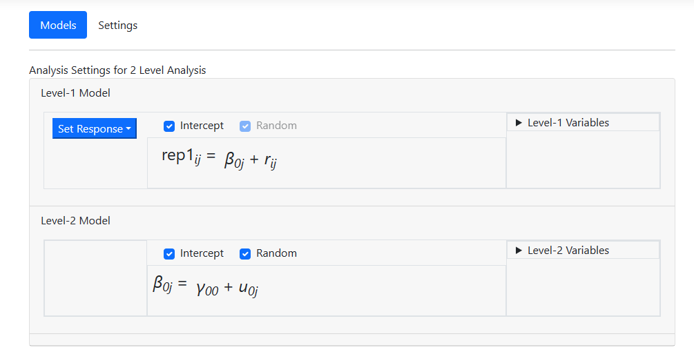 The next step is to include predictors in the model. At
level-1, we want to include the predictors MALE and PPED as uncentered
predictors. Open the Level-1 Variables field, and while holding the Control
button down, click on the two names. By default, these will be entered as
individual uncentered predictors as shown in the image below.
The next step is to include predictors in the model. At
level-1, we want to include the predictors MALE and PPED as uncentered
predictors. Open the Level-1 Variables field, and while holding the Control
button down, click on the two names. By default, these will be entered as
individual uncentered predictors as shown in the image below.
 Drag these variables into the level-1 equation before
releasing the mouse button. The model is updated again, and the level-1 model
specification is now complete.
Drag these variables into the level-1 equation before
releasing the mouse button. The model is updated again, and the level-1 model
specification is now complete.
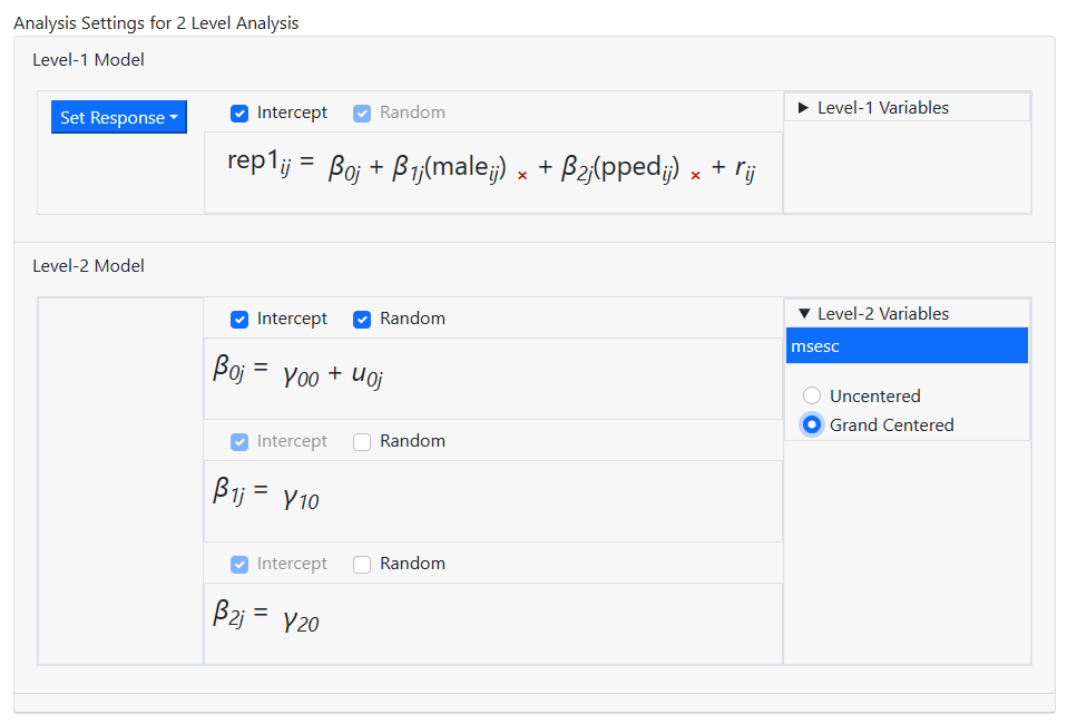
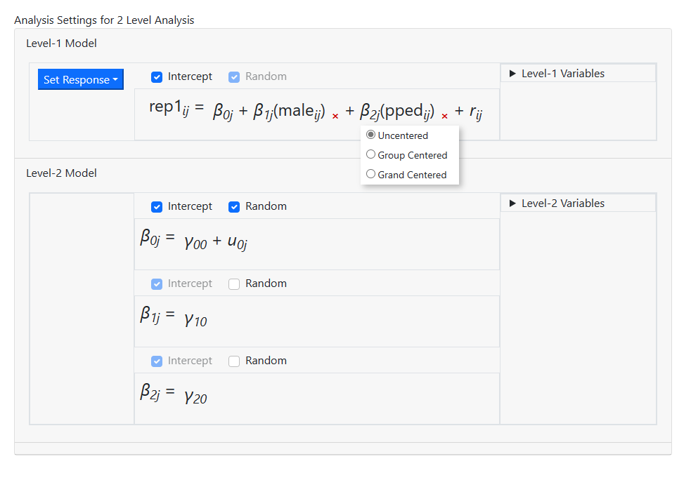 At level-2, the mean socio-economic status of the school has
to be added as a grand-mean centered variable. Open the Level-2 variables
field and select the variable MSESC, taking care to click grand centered before
dragging this variable into the intercept equation.
At level-2, the mean socio-economic status of the school has
to be added as a grand-mean centered variable. Open the Level-2 variables
field and select the variable MSESC, taking care to click grand centered before
dragging this variable into the intercept equation.
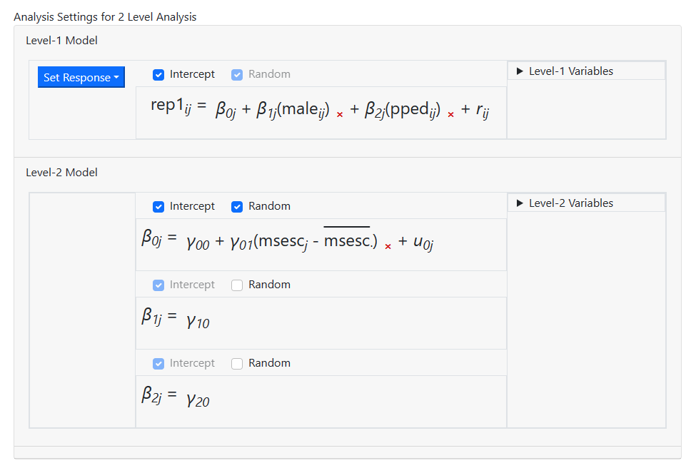
 The screen updates to the model shown below. This is the
model we intend to fit, so model building is now complete and we can move on to
the Settings page, where we can specify the distribution type and link
function. To do so, click on Settings at the top of the model page.
The screen updates to the model shown below. This is the
model we intend to fit, so model building is now complete and we can move on to
the Settings page, where we can specify the distribution type and link
function. To do so, click on Settings at the top of the model page.
Specifying the distribution type and link function
The program suggests a distribution type based on its reading of the data. For these data, it suggests the use of a Bernoulli model. The default link function for the Bernoulli model is the logit link function. As these suggested settings match our intentions, we make no changes on the Settings page. Analysis specification is now complete, and all that remains is to run the model.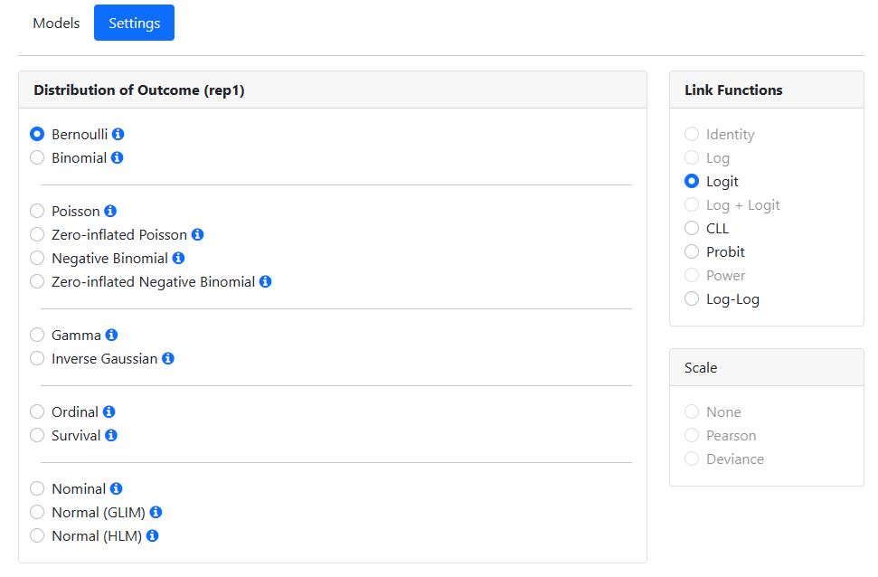
Running the model
To run the model, we move to the Run page, accessed by clicking on Run at the top of the window. When this page opens, only two options are available: saving the information on the model built in a MLCJSN file and running the syntax.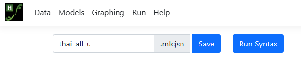 By default, the program will assign the same file name to
the MLCJSN file as that of the data file read in, in this case thai_all_u.
To save this analysis for potential reuse, we opt to save it using the Save
option under the name thai_bern.mlcjsn before clicking Run Syntax
to instruct the program to perform the analysis.
By default, the program will assign the same file name to
the MLCJSN file as that of the data file read in, in this case thai_all_u.
To save this analysis for potential reuse, we opt to save it using the Save
option under the name thai_bern.mlcjsn before clicking Run Syntax
to instruct the program to perform the analysis.
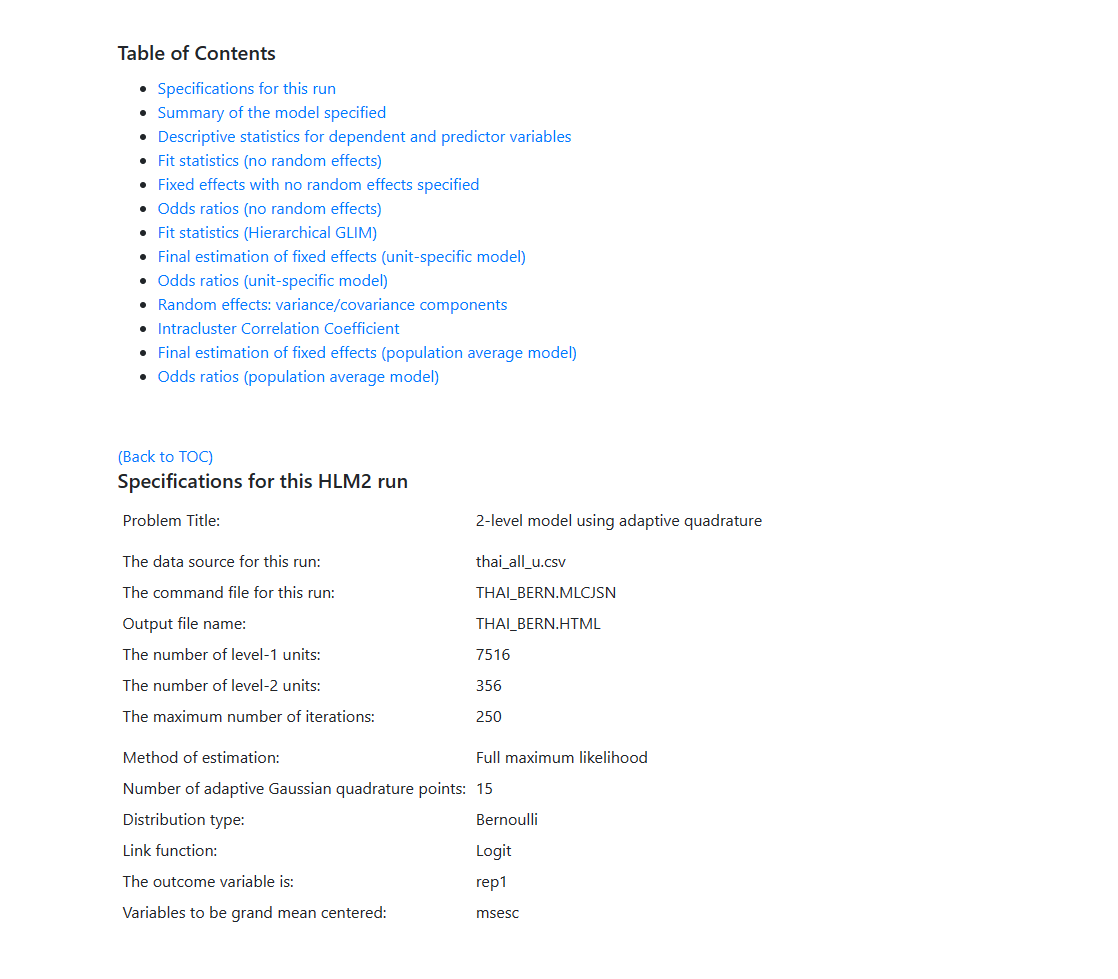
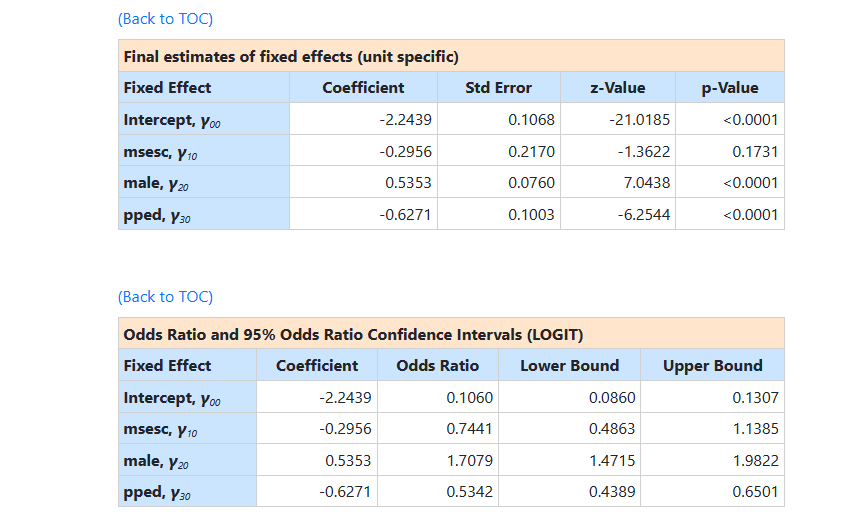
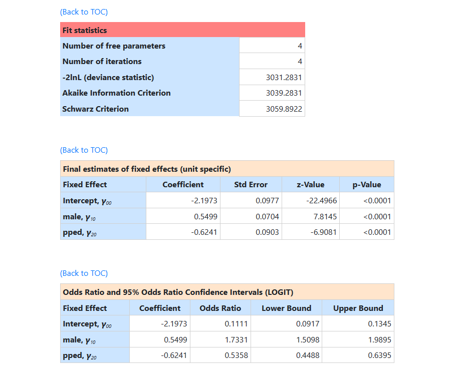
 For this model, the following results were obtained. The model
specifications and descriptive statistics are given first. Note that
descriptive statistics are given for both categories of the outcome variable (rep11 and
rep12).
For this model, the following results were obtained. The model
specifications and descriptive statistics are given first. Note that
descriptive statistics are given for both categories of the outcome variable (rep11 and
rep12).
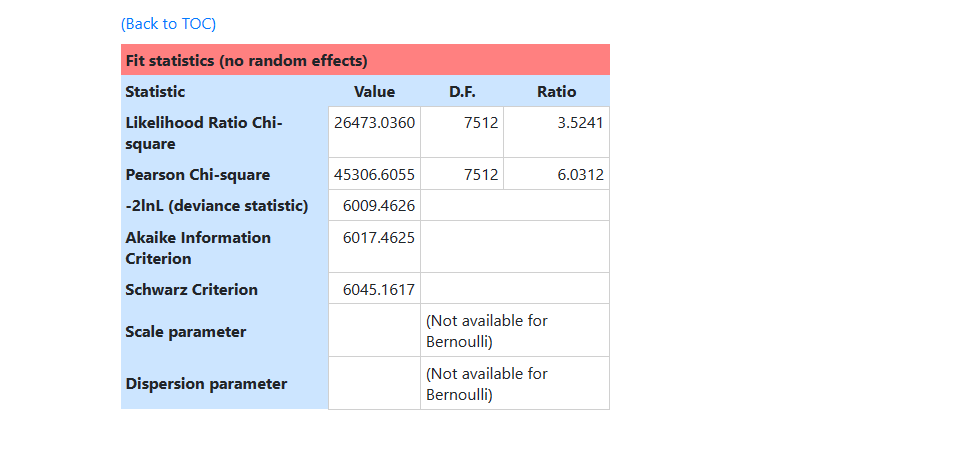
 This is followed by results and fit statistics for the model
without any random effects.
This is followed by results and fit statistics for the model
without any random effects.
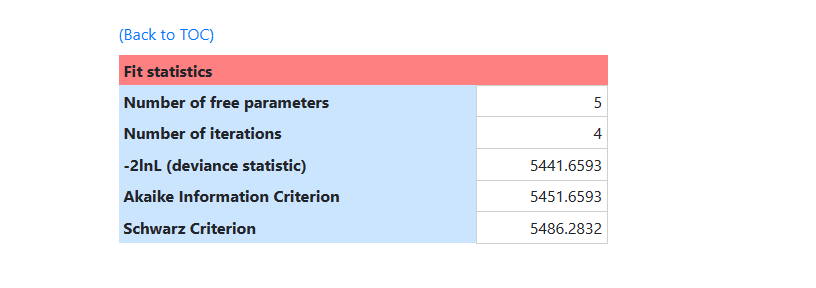
 In the next section, fit statistics at convergence are
reported:
In the next section, fit statistics at convergence are
reported:
 For models with non-continuous outcomes marginal (population
average) or conditional (subject-specific or unit specific) estimates can be
obtained.
For models with non-continuous outcomes marginal (population
average) or conditional (subject-specific or unit specific) estimates can be
obtained.
- The population average estimates are estimates of the regression coefficient for a person-level predictor which assumes the baseline value is the same for all individuals (i.e., averages over all the individuals).
- In contrast, the unit specific estimates represent the expected value of the regression coefficient for a person-level predictor assuming the effects of predictors vary across individuals and allowing individuals to have a different baseline value (effects are conditioned on the intercept variance).
 The results for random
effects in the model follow next. The program automatically also reports an
intra-cluster correlation coefficient if there is no more than one random
effect at each level of the hierarchy.
The results for random
effects in the model follow next. The program automatically also reports an
intra-cluster correlation coefficient if there is no more than one random
effect at each level of the hierarchy.
 It is assumed that the level-1 error variance is equal to π2/3 for the logit
link function if the model is true (see, e.g., Hedeker & Gibbons (2006), p.
157). Using this approximation, the formulae for the standard ICCs can
be adjusted.
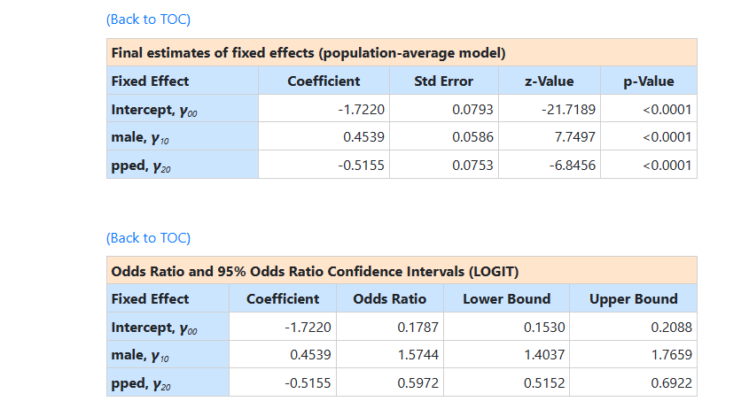
This is followed by the second set of final results, namely the population average results.
It is assumed that the level-1 error variance is equal to π2/3 for the logit
link function if the model is true (see, e.g., Hedeker & Gibbons (2006), p.
157). Using this approximation, the formulae for the standard ICCs can
be adjusted.
This is followed by the second set of final results, namely the population average results.
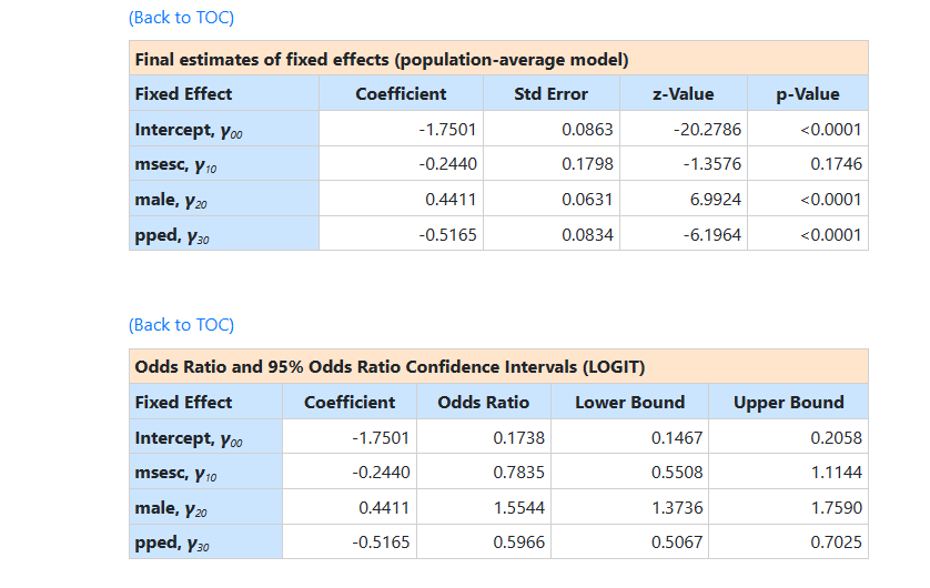 The two sets of results are very similar apart from the
estimate of the intercept coefficient. In the population average model the
intercept represents the expected log-odds of repetition for a person with
values of zero on the predictors (and therefore, for a female without
pre-primary experience attending a school of average SES. In the
unit specific results, the intercept is the expected log-odds of repetition
rate for the same kind of student, but one who attends a school that not only
has a mean SES of 0, but also has a random effect of zero (that is, a school with a
“typical” repetition rate for the school of its type).
The estimated intercept in the population average model is
-1.7501, which is the average logit. The estimated coefficients associated with
gender is 0.4411, which indicates that the
male respondents (MALE = 1) have a larger
The two sets of results are very similar apart from the
estimate of the intercept coefficient. In the population average model the
intercept represents the expected log-odds of repetition for a person with
values of zero on the predictors (and therefore, for a female without
pre-primary experience attending a school of average SES. In the
unit specific results, the intercept is the expected log-odds of repetition
rate for the same kind of student, but one who attends a school that not only
has a mean SES of 0, but also has a random effect of zero (that is, a school with a
“typical” repetition rate for the school of its type).
The estimated intercept in the population average model is
-1.7501, which is the average logit. The estimated coefficients associated with
gender is 0.4411, which indicates that the
male respondents (MALE = 1) have a larger  .
The estimate for the indicator of pre-primary education shows that students with
pre-primary education have a lower value.
To describe the ’s in a more accessible way to readers of reports, we
need the link functions to transform them into probabilities.
First, we substitute the regression weights and obtain the
function for
.
The estimate for the indicator of pre-primary education shows that students with
pre-primary education have a lower value.
To describe the ’s in a more accessible way to readers of reports, we
need the link functions to transform them into probabilities.
First, we substitute the regression weights and obtain the
function for 
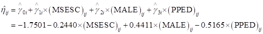 Recall that the mean value of MSESC over schools was zero. We
can thus use the expression above to calculate
for the four
groups of students formed by the cross-classification of gender by pre-primary
education at a mean value of MSESC.
Recall that the mean value of MSESC over schools was zero. We
can thus use the expression above to calculate
for the four
groups of students formed by the cross-classification of gender by pre-primary
education at a mean value of MSESC.
| Group | |
|---|---|
| Males with pre-primary education | -1.8255 |
| Males without pre-primary education | -1.3090 |
| Females with pre-primary education | -2.2666 |
| Females without pre-primary education | -1.7482 |
’s into corresponding probabilities by using the logit
link function:
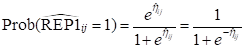
| Group |  |
|---|---|
| Males with pre-primary education | 0.1388 |
| Males without pre-primary education | 0.2127 |
| Females with pre-primary education | 0.0939 |
| Females without pre-primary education | 0.1480 |
| MSESC | Group | |
|---|---|---|
| MSESC = -0.77 | Males with pre-primary education0.1628 | |
| Males without pre-primary education | 0.2458 | |
| Females with pre-primary education | 0.1112 | |
| Females without pre-primary education | 0.1736 | |
| MSESC = 1.49 | Males with pre-primary education | 0.1007 |
| Males without pre-primary education | 0.1581 | |
| Females with pre-primary education | 0.0672 | |
| Females without pre-primary education | 0.1080 |
Binomial model with logit link function
The data
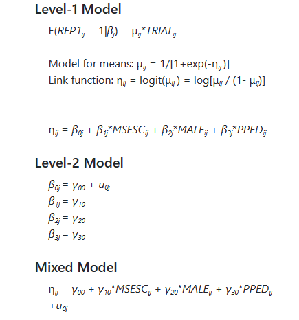
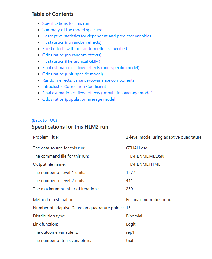
We again use the data from a national survey of primary education in Thailand (see Raudenbush & Bhumirat, 1992, for details), conducted in 1988. We again focus on the probability that a child will repeat a grade during the primary years. The first few lines of the data file GTHAI1.CSV are shown below. When the contents of this file is compared to that used for fitting the Bernoulli model, we see that in this case there seems to be fewer records associated with each SCHOOLID. A new variable, TRIAL, also appears in this file.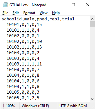 The variable TRIAL reports the number of observed repetitions within each of four cells,
formed by the cross-tabulation of the two binary variables MALE and PPED. For
each school, there may be a maximum of 4 lines of data, representing (MALE,
PPED) = (0, 1), (1,1), (0, 0) and (1,0).
The variable TRIAL reports the number of observed repetitions within each of four cells,
formed by the cross-tabulation of the two binary variables MALE and PPED. For
each school, there may be a maximum of 4 lines of data, representing (MALE,
PPED) = (0, 1), (1,1), (0, 0) and (1,0).
- REP1 indicates whether a grade was repeated (1 if yes, 0 if no).
- MALE indicates the gender of students within a cell, with 1 if the student is male and 0 if female.
- PPED = 1 if student in the cell had pre-primary experience. For students without pre-primary experience, PPED = 0.
- The number of trials is represented by the variable TRIAL.
The model
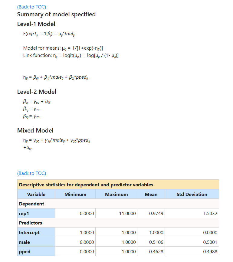
It is hypothesized that the child’s gender and pre-primary experience will be associated with the probability of repetition. Every level-1 record corresponds to a cell with students nested within it with the number of observed repetitions for the cell denoted by TRIAL. The sampling distribution of the Binomial distribution is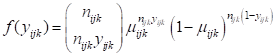 and the variance is
 The model we consider again uses the logit link function:
 The model for the means can be expressed as
 and in terms of our variables we can write it as shown below, also utilizing the variable
TRIAL to indicate the number of repetitions per cell.
and in terms of our variables we can write it as shown below, also utilizing the variable
TRIAL to indicate the number of repetitions per cell.
Reading the data
To start a new analysis, select the New Analysis option on the landing page. The Data page will open. As a first step, select the
data file gthai1.csv and click Open to obtain the image shown
below.
The Data page will open. As a first step, select the
data file gthai1.csv and click Open to obtain the image shown
below.
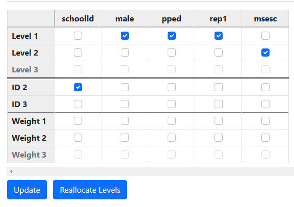
 Start by selecting the variable SCHOOLID as the variable
denoting the hierarchical structure by checking its box in the ID 2
line. Next, select all other variables in a similar way in the Variables
line of the second table as shown below.
Start by selecting the variable SCHOOLID as the variable
denoting the hierarchical structure by checking its box in the ID 2
line. Next, select all other variables in a similar way in the Variables
line of the second table as shown below.
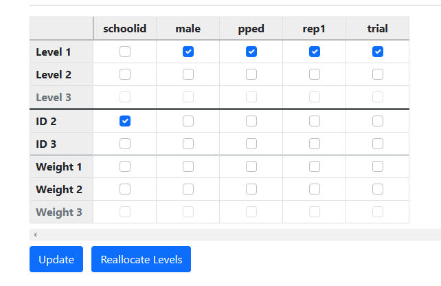
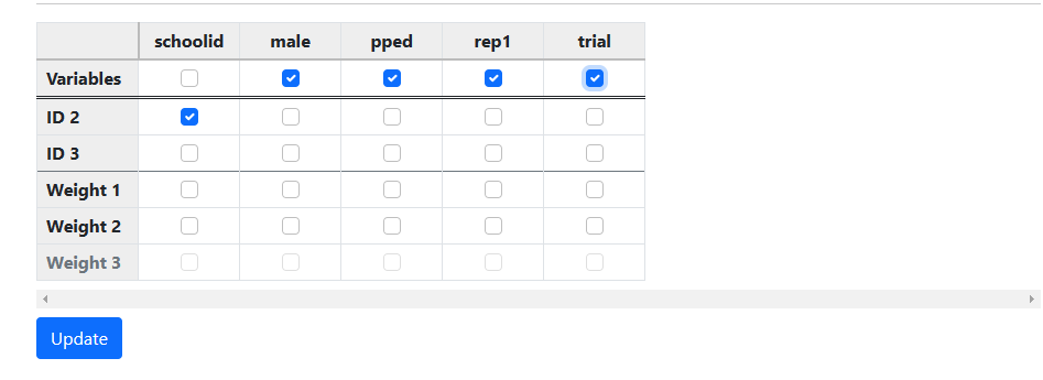 Click Update to prompt the automatic allocation
of variables to the different levels of the hierarchy.
Click Update to prompt the automatic allocation
of variables to the different levels of the hierarchy.
Model building
With data specification complete, model building can begin. To start, click on Models at the top of the window. Following the same steps as for the Bernoulli model, set up the model shown below.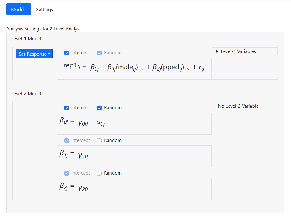
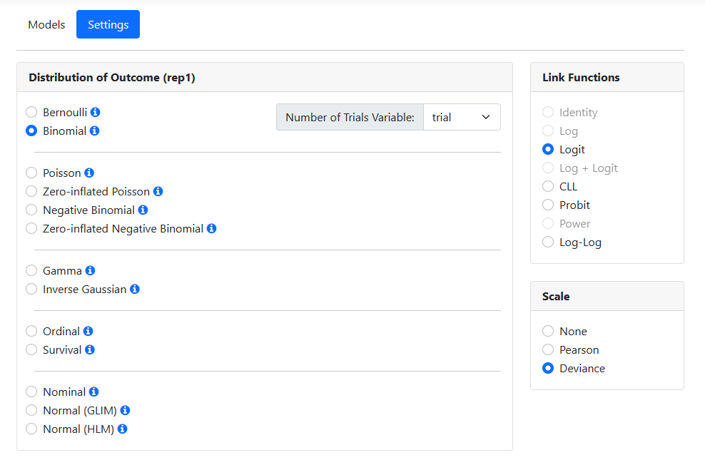
Specifying the distribution type and link function
The program suggests a distribution type based on its reading of the data. For these data, it suggests the use of a Poisson model. We need to make changes here, as we want to fit a Binomial model with logit link function to the data.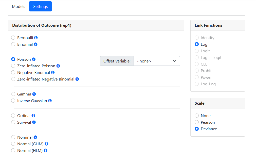 Change the Distribution of Outcome field to Binomial
by clicking the radio button for the Binomial model in the Distribution
of Outcome field. When updated, the Settings page shows that the
default link function for this model is the logit link function. We also
set the Number of Trials Variable by selecting the variable TRIAL from
the drop-down menu associated with this option. Analysis specification is now
complete, and all that remains is to run the model.
Change the Distribution of Outcome field to Binomial
by clicking the radio button for the Binomial model in the Distribution
of Outcome field. When updated, the Settings page shows that the
default link function for this model is the logit link function. We also
set the Number of Trials Variable by selecting the variable TRIAL from
the drop-down menu associated with this option. Analysis specification is now
complete, and all that remains is to run the model.
Running the model
We move to the Run page by clicking on Run at the top of the window. When this page opens, only two options are available: saving the information on the model built in a MLCJSN file and running the syntax. By default, the program will assign the same file name to
the MLCJSN file as that of the data file read in, in this case gthai1.
To save this analysis for potential reuse, we opt to save it using the Save
option under the name thai_bnml.mlcjsn before clicking Run Syntax
to instruct the program to perform the analysis.
By default, the program will assign the same file name to
the MLCJSN file as that of the data file read in, in this case gthai1.
To save this analysis for potential reuse, we opt to save it using the Save
option under the name thai_bnml.mlcjsn before clicking Run Syntax
to instruct the program to perform the analysis.
 For this model, the following results were obtained. The
model specifications and descriptive statistics are given first. Note that
descriptive statistics are given for both categories of the outcome variable (rep11 and rep12).
For this model, the following results were obtained. The
model specifications and descriptive statistics are given first. Note that
descriptive statistics are given for both categories of the outcome variable (rep11 and rep12).
 This is followed by results and fit statistics for the model
without any random effects.
This is followed by results and fit statistics for the model
without any random effects.
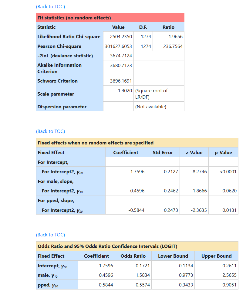 The fit statistics at convergence follows, followed by the final unit specific results.
 Information on the variance components is given next. The intracluster correlation coefficient is also
provided.
Information on the variance components is given next. The intracluster correlation coefficient is also
provided.
 Finally, final population average results are reported.
 The two sets of results are very similar apart from the
estimate of the intercept coefficient. The estimated intercept in the
population average model is -1.7220, which is the average logit. The estimated
coefficients associated with gender (MALE) is 0.4539, which indicates that the male respondents (MALE = 1) have a
larger
The two sets of results are very similar apart from the
estimate of the intercept coefficient. The estimated intercept in the
population average model is -1.7220, which is the average logit. The estimated
coefficients associated with gender (MALE) is 0.4539, which indicates that the male respondents (MALE = 1) have a
larger  . The estimate for the indicator of pre-primary education (PPED)
shows that students with pre-primary education have a lower
. The estimate for the indicator of pre-primary education (PPED)
shows that students with pre-primary education have a lower  value. Females
with pre-primary education again have the lowest
value. Females
with pre-primary education again have the lowest  value.