Setting up a moderation analysis with the HSB data
The program can fit three different
moderation models. In this example, we show how to set up the simplest of the three
moderation models, with a focal variable and a single moderator variable, using
the well-known HSB data.
 The following topics are covered in this document:
Description of the
data and the model
Reading in the data
Model building
Defining outcome type and other options
Requesting graphs
Running the model
The following topics are covered in this document:
Description of the
data and the model
Reading in the data
Model building
Defining outcome type and other options
Requesting graphs
Running the model
The data
The High School and Beyond (HSB) survey is a nationally representative sample of U.S. public
and Catholic high schools.The data file used here contains
information on 7185 students from 160 schools. Of these schools, 90 were public
schools and 70 Catholic schools.
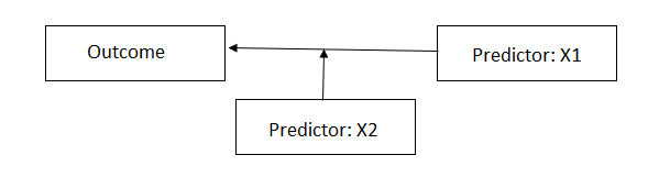
Here we fit a model related to those given in Hierarchical Linear Models,
Raudenbush & Bryk (2002). We wish to examine the relationship between student
socio-economic status (SES) and student mathematics achievement (MATHACH),
while also evaluating the extent to which the sector a school originates from
(public vs Catholic) moderates the relationship between SES and mathematics
achievement.
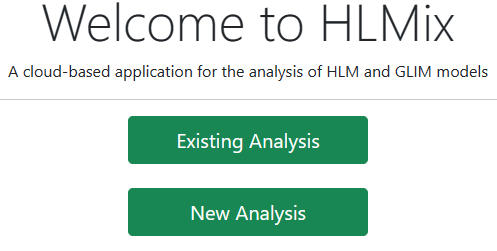
 To start a new analysis, select the New Analysis option on the landing page.
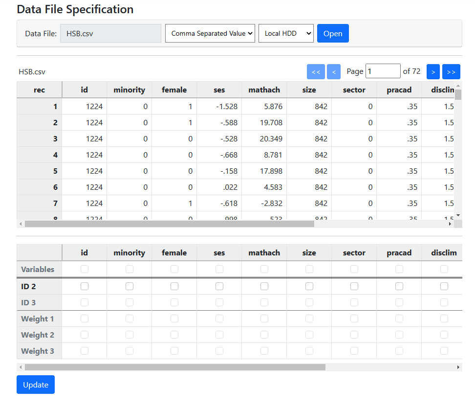
 The Data page will open. As a first step, select the
data file HSB.csv and click Open to obtain the image shown below.
Note that the data file may reside on a local hard drive, OneDrive, or Google
Drive. A description of the variables contained in the data file are given
below the image.
The Data page will open. As a first step, select the
data file HSB.csv and click Open to obtain the image shown below.
Note that the data file may reside on a local hard drive, OneDrive, or Google
Drive. A description of the variables contained in the data file are given
below the image.
 The variables are:
-
ID indicates the school number and serves as our level-2 ID in
this example
-
MATHACH, a measure of mathematics achievement. serving as outcome
variable in this example
-
MINORITY is an indicator for student ethnicity (1 = minority, 0 =
other)
-
FEMALE is an indicator for student gender (1 = female, 0 = male)
-
SES is a standardized scale constructed from variables measuring
parental education, occupation, and income. This is a measure of the
student’s socio-economic status
-
SIZE is an indicator of school enrollment
-
SECTOR is an indicator variable that assumes the value of 1 for
Catholic schools, and 0 for public schools
-
PRACAD indicates the proportion of students in the academic track in a specific school
-
DISCLIM is a scale measuring disciplinary climate in a school
HIMNTY represents the percentage minority enrollment and is coded 1 for schools
with more than 40% minority enrollment, and 0 for those with less than 40%
-
MEANSES measures the mean of the SES
values for the students in a specific school
In the current example, we will only be using the variable
MATHACH, SES and SECTOR, along with the ID variable.
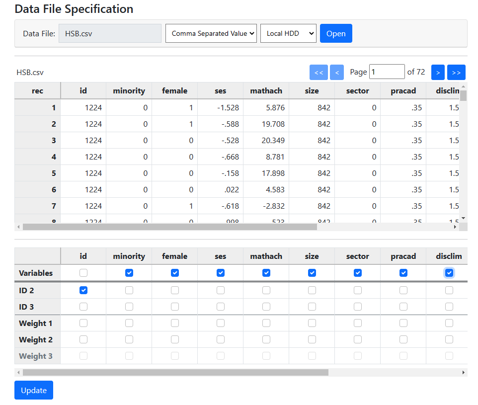
The first step in data file specification is to identify the
ID variable or variables. In this example, we are looking at a two-level model
and need to specify only a level-2 ID. This ID is represented by the variable
appropriately, if unimaginatively, named “id”. Check the box for
this in the ID 2 row of the second table.
After doing so, select all variables that may be used in
model building. Here, all the variables have been checked in the Variables
row of the second table. Once all variables have been selected, click Update
to request the program to automatically assign the selected variables to the
different levels of the hierarchy.
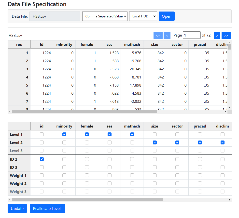
 The program has identified the variables MINORITY, FEMALE, SES,
and MATHACH as level-1 variables, in other words, student characteristics. The
variables SIZE, SECTOR, PRACAD, and DISCLIM are school level variables and are
appropriately indicated as level-2 variables.
The program has identified the variables MINORITY, FEMALE, SES,
and MATHACH as level-1 variables, in other words, student characteristics. The
variables SIZE, SECTOR, PRACAD, and DISCLIM are school level variables and are
appropriately indicated as level-2 variables.
Model building
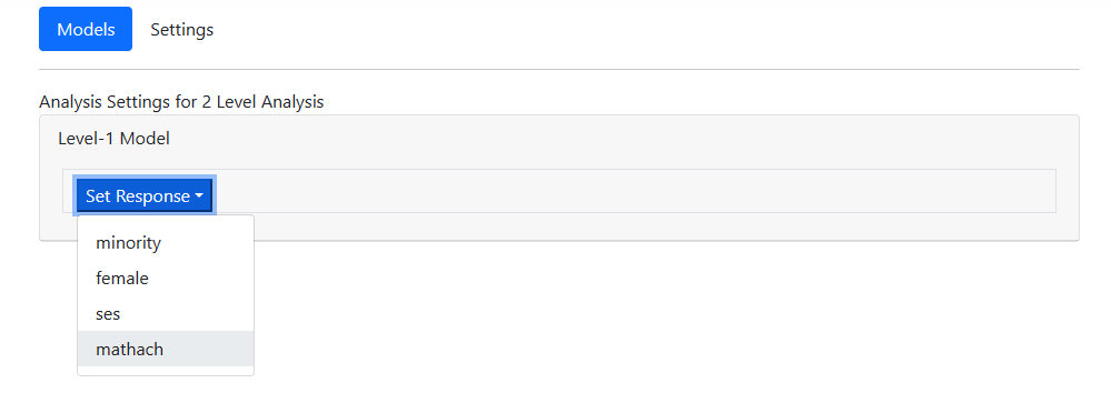
Data file specification is now complete, and model building
can start. To begin, click on the Models link at the top of the page to
open the Models page. When first opened, only one option is available in
the Level-1 Model field: Set Response. Use the drop-down list
associated with Set Response to select the outcome variable of choice,
in this case MATHACH.
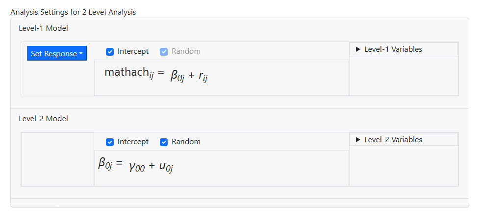
 On selection of the outcome
variable, the page is automatically updated and now displays a fully
unconditional model with MATHACH as outcome.
On selection of the outcome
variable, the page is automatically updated and now displays a fully
unconditional model with MATHACH as outcome.
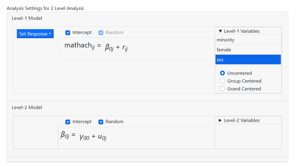
 To add predictors to the model,
the Level-1 Variables and Level-2 Variables fields are used.
Start by clicking on the Level-1 Variables field and selecting the
variable SES, as shown below. Note that a variable can be entered as either
uncentered, group centered (that is, centered around the group mean of the
level-2 unit a level-1 record is nested in) or grand centered (in other words,
centered around the mean of the variable over all level-1 records, irrespective
of the unit a level-1 record is nested in). In this simple example, we enter
SES as an uncentered predictor to the model by dragging the variable name SES
from the Level-1 Variables field into the equation for MATHACH.
To add predictors to the model,
the Level-1 Variables and Level-2 Variables fields are used.
Start by clicking on the Level-1 Variables field and selecting the
variable SES, as shown below. Note that a variable can be entered as either
uncentered, group centered (that is, centered around the group mean of the
level-2 unit a level-1 record is nested in) or grand centered (in other words,
centered around the mean of the variable over all level-1 records, irrespective
of the unit a level-1 record is nested in). In this simple example, we enter
SES as an uncentered predictor to the model by dragging the variable name SES
from the Level-1 Variables field into the equation for MATHACH.
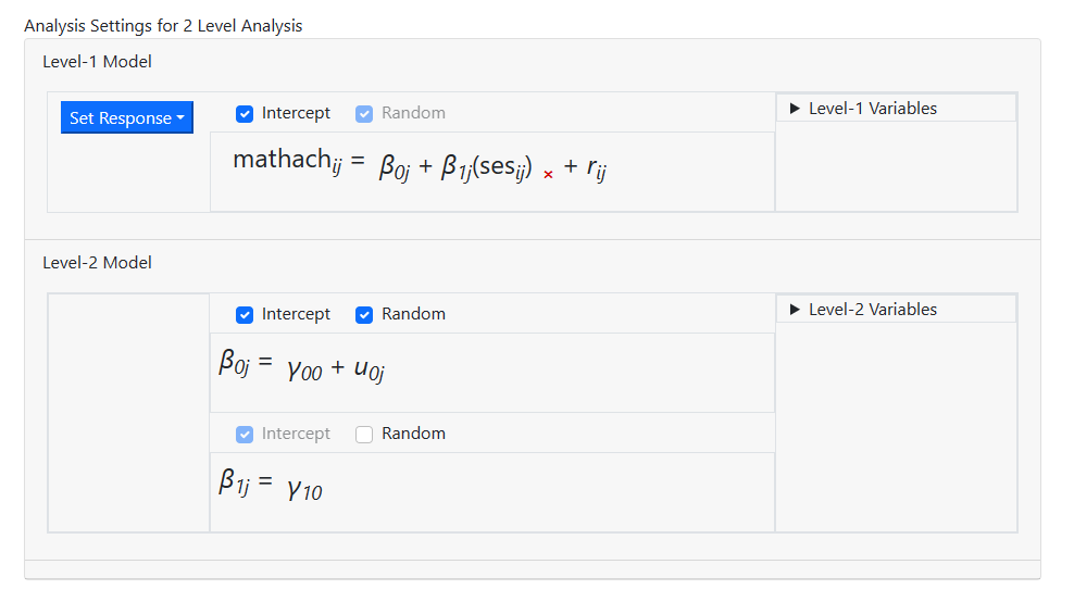
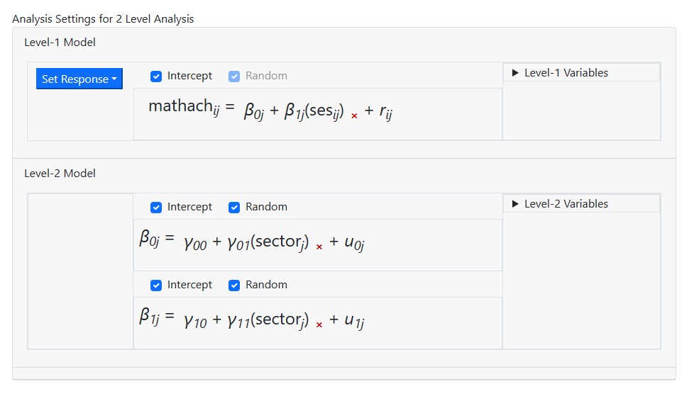
 The page now displays a random intercept model, with MATHACH
as outcome, a fixed and random intercept coefficient, and a fixed SES slope
coefficient.
The page now displays a random intercept model, with MATHACH
as outcome, a fixed and random intercept coefficient, and a fixed SES slope
coefficient.
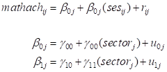
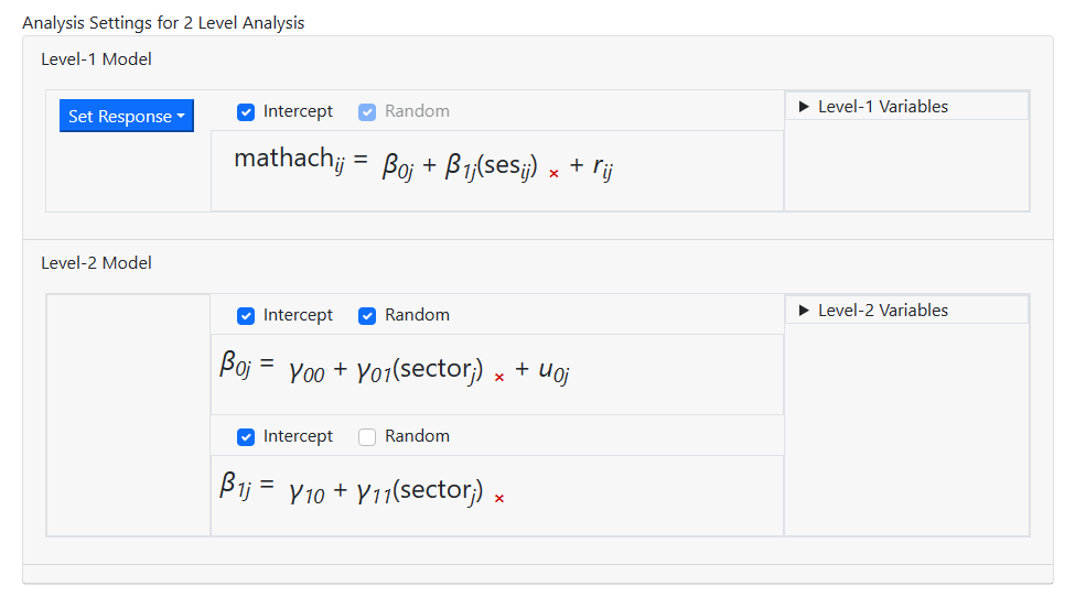
 We now add the level-2 variable SECTOR to both of the
level-2 equations by selecting it from the Level-2 Variables field and
dragging it into both the level-2 equations. This model contains a fixed and
random intercept term, fixed coefficients for SES and SECTOR, and a fixed
coefficient for the interaction between SES and SECTOR. The latter is created
by adding the variable SECTOR to the SES slope equation.
We now add the level-2 variable SECTOR to both of the
level-2 equations by selecting it from the Level-2 Variables field and
dragging it into both the level-2 equations. This model contains a fixed and
random intercept term, fixed coefficients for SES and SECTOR, and a fixed
coefficient for the interaction between SES and SECTOR. The latter is created
by adding the variable SECTOR to the SES slope equation.
 As a final step, check the Random check box for the
second level-2 equation to also include a random SES slope coefficient. In
other words, both intercept and SES slope are now allowed to vary randomly over
the schools at level-2.
As a final step, check the Random check box for the
second level-2 equation to also include a random SES slope coefficient. In
other words, both intercept and SES slope are now allowed to vary randomly over
the schools at level-2.
Defining the outcome type
Our Models page is now
complete, and we can move on the specifying additional options such as the type
of outcome variable on the Settings page. The Settings page is
accessed by clicking on the Settings button.
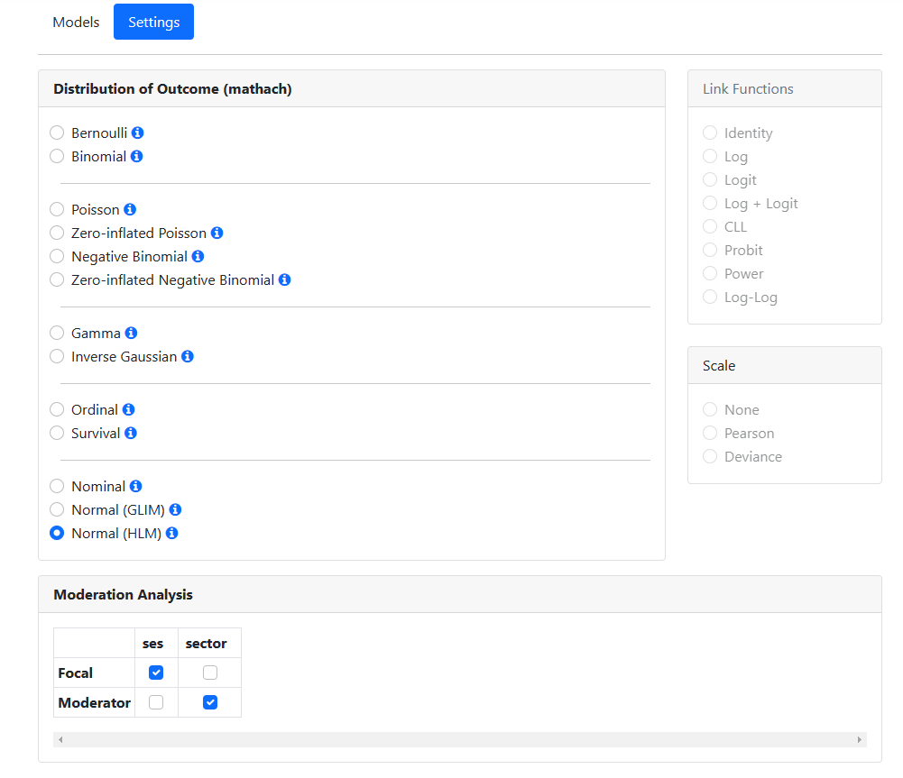
Our outcome variable MATHACH
is a continous normally distributed variable, and the program will by default
attempt to guide the user to the most appropriate choice of outcome
distribution, in this case Normal (HLM). Currently, moderation analyses
can only be performed for a normal (HLM) model, so we need not change the
distribution of the outcome.
At the bottom of the page, an
Moderation Analysis section is displayed if the program picks up that
interaction terms permitting moderation analysis have been specified on the Models
page. Recall that we created a cross-level interaction between the level-1
variable SES and the level-2 variable SECTOR by adding SECTOR to the equation
for the SES slope. As a result, we now can opt to select a focal variable and a
moderator variable. As we want to evaluate the impact of the second level
predictor SECTOR on the relationship between MATHACH and SES, we select SES as
the focal variable and SECTOR as the moderator variable in the Interactions
field.
Requesting graphs
For moderation analyses, two types of graphs may be made. By
default, both simple slopes and confidence interval graphs will be produced
with default graph settings. To modify the graph parameters, the Graphing
page is used. Open the Graphing page by clicking on Graphing at
the top of the page.
Note that you can request either a Simple slope
graph, a Confidence interval graph, or both.
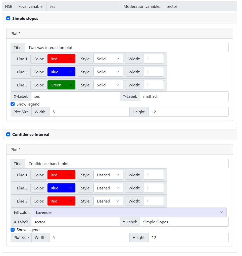 The color, style and line
width may be changed, along with the color a line is to be displayed in. One
can opt to show or suppress a legend, and change graph tile and the axes
labels. In the case of a confidence graph, an additional option is available to
set the fill color for the area between the two confidence intervals lines.
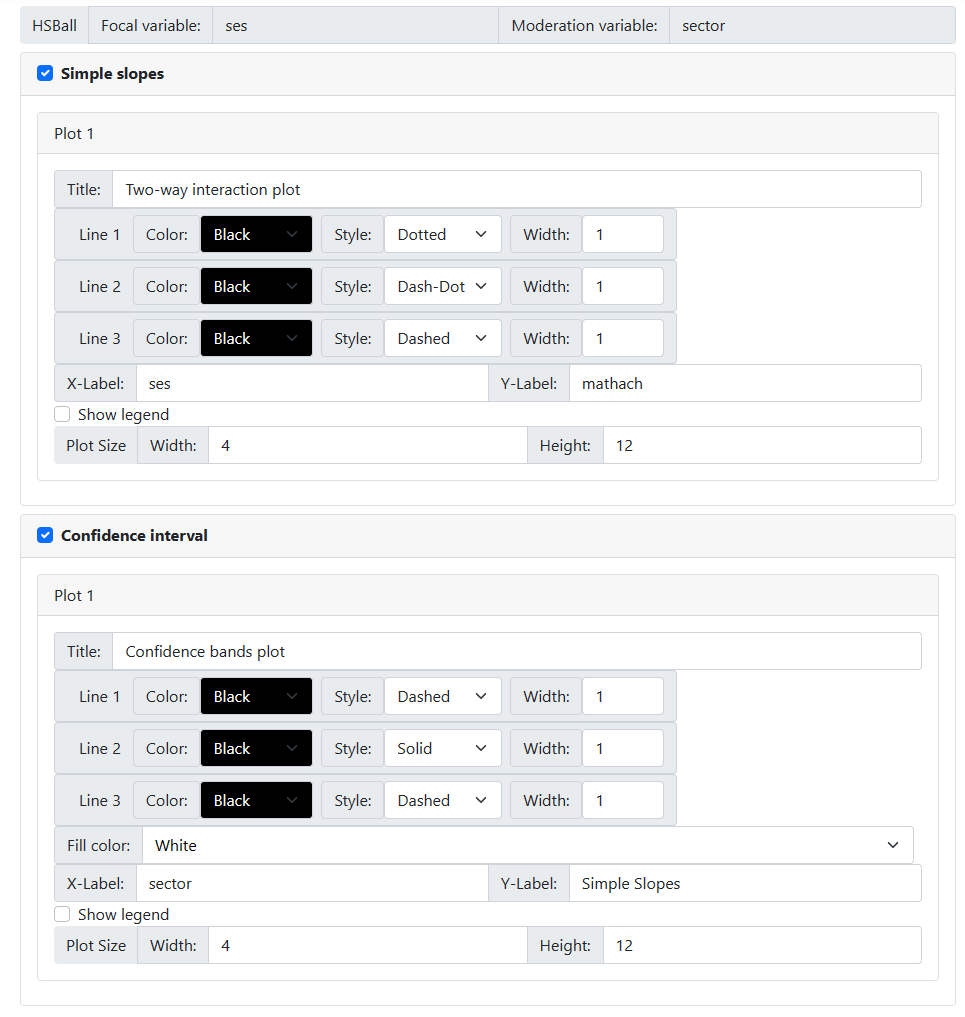
Assuming that a black and
white graph would be best for publication purposes, we opted for the settings
shown below.
The color, style and line
width may be changed, along with the color a line is to be displayed in. One
can opt to show or suppress a legend, and change graph tile and the axes
labels. In the case of a confidence graph, an additional option is available to
set the fill color for the area between the two confidence intervals lines.
Assuming that a black and
white graph would be best for publication purposes, we opted for the settings
shown below.
Running the model
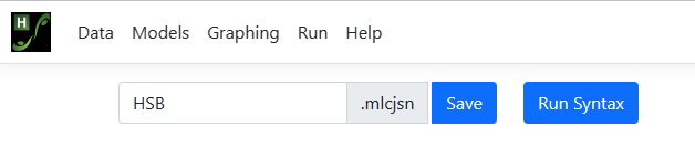
After specifying the appearance of the moderation graphs,
click on the Run option on the top of the page to run the analysis and
graphs. Click the Run Syntax button to start the analysis.
 The Progress window opens. Error messages
concerning the analysis, if applicable, will also appear here. The information
in this window can be copied to a clipboard to by using the Copy to
Clipboard button at bottom left. Close the Progress window by
clicking Close to return to the Run page. The Run page will display links to all output files.
The Progress window opens. Error messages
concerning the analysis, if applicable, will also appear here. The information
in this window can be copied to a clipboard to by using the Copy to
Clipboard button at bottom left. Close the Progress window by
clicking Close to return to the Run page. The Run page will display links to all output files.
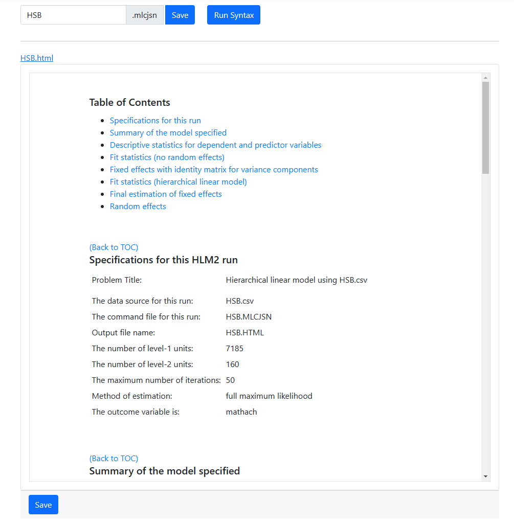
 For example, clicking the link to the HTML output will display this output in a window on the
Run Page:
For example, clicking the link to the HTML output will display this output in a window on the
Run Page:
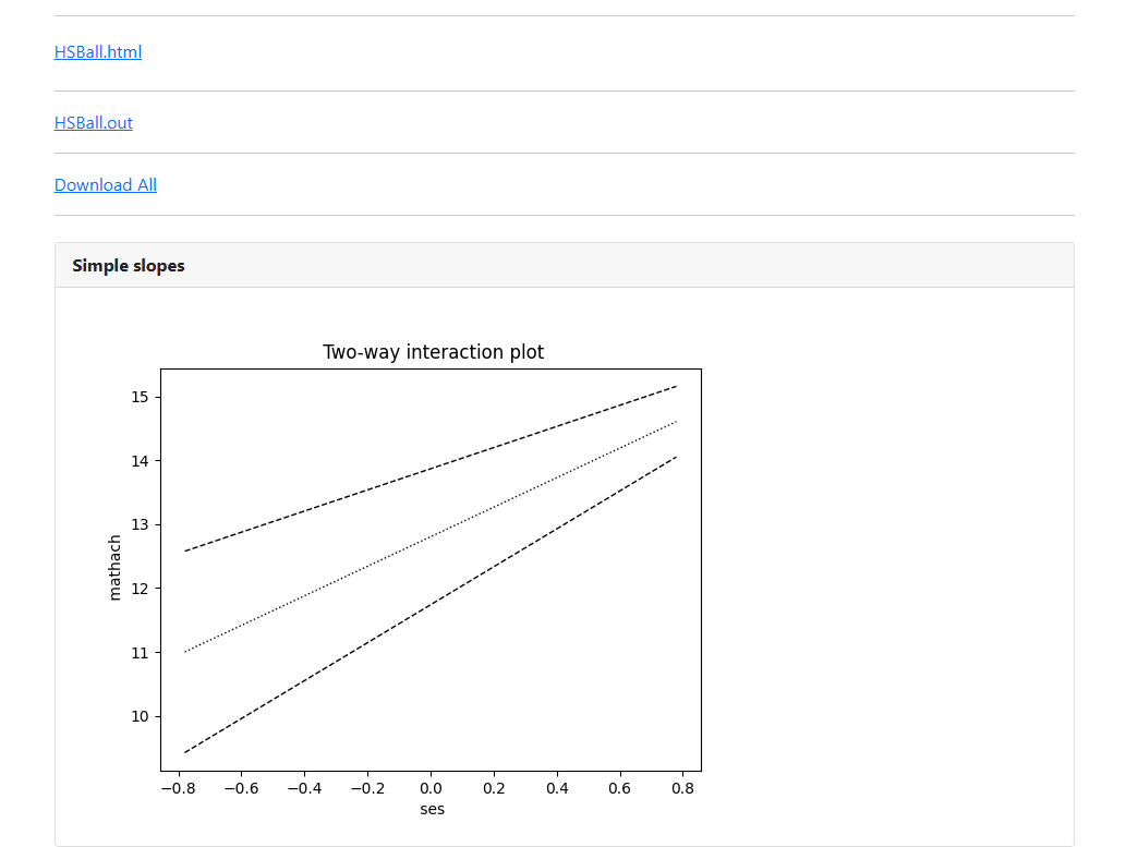
 The graphs requested are also displayed on the Run
page in the browser. From here, they can be copied and pasted into any word
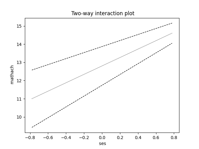
processing program. The two graphs are shown below.
The first of the available graphs is a plot of the conditional regression line(s) describing the relationship between the outcome and the focal predictor as a function of the moderator. The plot will automatically show a line at each of three values of the moderator variable: mean – 1 standard deviation, mean, and mean + 1 standard deviation. In other words, the value of the moderator variable is held constant at three specific values. Values of the focal variable are used to define the x-axis, and the plot is confined to the area (mean of focal variable – 2 standard deviations, mean of focal variable + 2 standard deviations).
The graphs requested are also displayed on the Run
page in the browser. From here, they can be copied and pasted into any word
processing program. The two graphs are shown below.
The first of the available graphs is a plot of the conditional regression line(s) describing the relationship between the outcome and the focal predictor as a function of the moderator. The plot will automatically show a line at each of three values of the moderator variable: mean – 1 standard deviation, mean, and mean + 1 standard deviation. In other words, the value of the moderator variable is held constant at three specific values. Values of the focal variable are used to define the x-axis, and the plot is confined to the area (mean of focal variable – 2 standard deviations, mean of focal variable + 2 standard deviations).
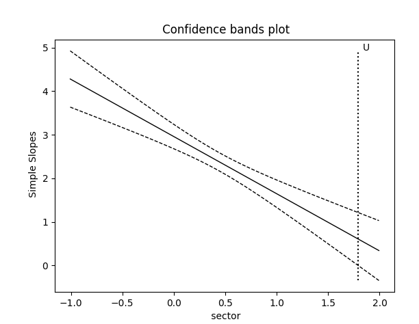
 The second graph shows the regression line describing the
relationship between the outcome and the focal predictor as a function of the
moderator, along with a 95% confidence interval. It also shows the so-called
region of significance, provided that the boundaries of this region fall within
the scale set by the values of the moderator variable, which again defines the
x-axis. The region between the lower and upper bound of the region of
significance indicates the values of the moderator for which the slope of the
regression of outcome on focal variable transitions from non-significance to
significance. In the current example, only the lower bound, denoted by
“L” on the graph, falls within the scale set by the moderator
variable values.
The second graph shows the regression line describing the
relationship between the outcome and the focal predictor as a function of the
moderator, along with a 95% confidence interval. It also shows the so-called
region of significance, provided that the boundaries of this region fall within
the scale set by the values of the moderator variable, which again defines the
x-axis. The region between the lower and upper bound of the region of
significance indicates the values of the moderator for which the slope of the
regression of outcome on focal variable transitions from non-significance to
significance. In the current example, only the lower bound, denoted by
“L” on the graph, falls within the scale set by the moderator
variable values.