Two-level centered model for the HSB data
In this example, we use the data from the High School and
Beyond Study of 1982 and set up a model closely following some of the models in
Chapter 4 of the well-known Raudenbush & Bryk (Sage, 2nd
Edition) text. Here we concentrate on how to set up the analysis, but readers
are strongly urged to also read the relevant chapter to gain more insight into
the model design decisions and interpretation of results obtained.
Description
of the data
The model
Reading in the data
Model
building
Defining outcome type and other options
Running the model
Description of the data
Data were available for a subsample of students and schools
surveyed in 1982. The sample includes information on 160 schools, with a total
of 7185 students nested within these. At a school level, we have the following
information:
-
Type of school, as represented by the variable
SECTOR. This variable assumes values of either 0 or 1, indicating whether the
school is a public or Catholic school.
-
A measure of the average socio-economic status
of students within each school, represented by the variable MEANSES.
For each student, we have information on
-
A standardized measure of mathematical
achievement (MATHACH)
-
The student’s socio-economic status (SES).
This measure is a composite of parental education and occupation and the income
of the household.
-
With the students nested within a school, we define the
lowest level of the hierarchy as the student level, and the second level as the
school level. The focus here is to determine to what extent schools differ in
the mean mathematics achievement, taking both socio-economic status and school
sector (SECTOR) into account.
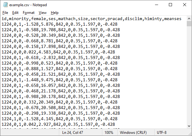
The data are stored in the file example.csv. The first
few lines of this comma-separated values file are shown below.
The first line of the file contains the variable
names.
Each subsequent line contains information for a
student. The file contains additional variables as well, such as FEMALE,
representing the gender of a student.
The first column, ID, contains the ID number of
the school a student belongs to. This is followed by all student level
information and all school level information for the school in question. Here
we are looking at data from school with ID = 1224.
School level information for this school, for
example the information on SECTOR and MEANSES, are appended to the record for
each student in the school.
It is easy to see that while
student level variables such as MATHACH changes from student to student, values
for school level variables such as MEANSES stays the same over all students
within the school.
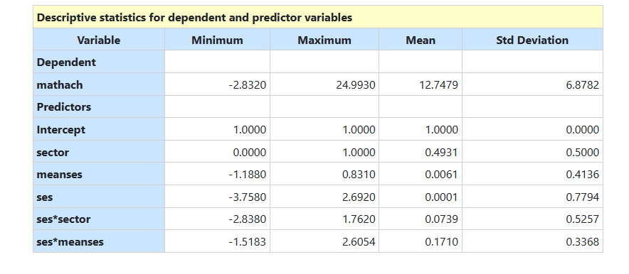
 Descriptive statistics for variables of interest in this
example are shown below.
Descriptive statistics for variables of interest in this
example are shown below.
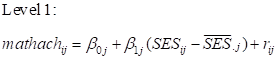
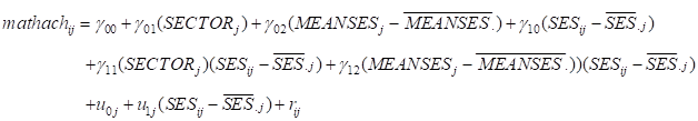
The model
The model we want to fit is the following:
 and
and
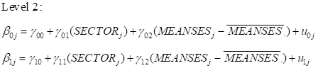 A variable with a horizontal bar on top represents the grand mean unless it contains a subscript
such as .j in which case it represents a group mean.
The model can also be written as a mixed model of the form
A variable with a horizontal bar on top represents the grand mean unless it contains a subscript
such as .j in which case it represents a group mean.
The model can also be written as a mixed model of the form
 The
The  coefficients represent the fixed effects in the model, while
 and
and
 represent the random intercept and random slope effects. Residual variation at level-1 is
represented by
represent the random intercept and random slope effects. Residual variation at level-1 is
represented by
 .
It is assumed
.
It is assumed
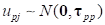 and
and

Reading in the data
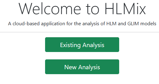
The first step is to read the data into the program. This
can be done in one of two ways:
-
Clicking New Analysis on the landing page, which will take you to the Data page.
-
Clicking on the Data link at the top of the window.
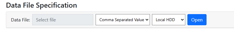
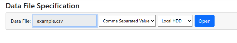
 When first accessed, the Data page shows the following fields:
-
Select file: used to provide the name of the data file
-
Type of file: by default, it is assumed
that comma-separated value files (CSV) will be used. In subsequent versions of
the program, this menu will be extended to allow other types of data files as
well.
-
Location of file: by default, it is
assumed that the file is stored on a local hard disk drive (HDD). However, one
could access files stored on One Drive or Google Drive too.
 The data set used here is a CSV file stored on the local
hard disk drive, so it is only necessary to click in the Select file to
start the process of data specification. Clicking in this field will open a
standard Windows Open dialog box, allowing the user to browse for the
file. After selection, the Data page is updated to
The data set used here is a CSV file stored on the local
hard disk drive, so it is only necessary to click in the Select file to
start the process of data specification. Clicking in this field will open a
standard Windows Open dialog box, allowing the user to browse for the
file. After selection, the Data page is updated to
 Clicking the Open button requests the program to open
the file and display its contents:
Clicking the Open button requests the program to open
the file and display its contents:
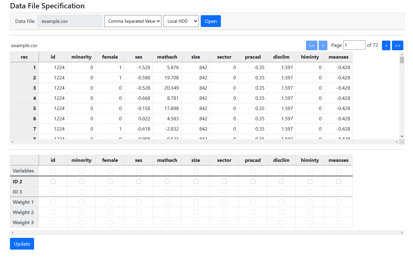 The contents of the data file are displayed in the first of
the two tables on the page. Note that all the data are accessible –
simply use the scroll bars and > and >> buttons to
access any part of the data set.
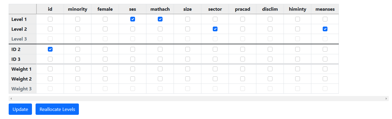
The second table needs to be completed before model
specification can take place. Information required includes the following:
The contents of the data file are displayed in the first of
the two tables on the page. Note that all the data are accessible –
simply use the scroll bars and > and >> buttons to
access any part of the data set.
The second table needs to be completed before model
specification can take place. Information required includes the following:
-
ID variable(s): The second and third line
of check boxes are used to identify these. Note that only the ID2 line
is active at the start, prompting the user to first select the level-2 ID. Once
that is done, selection of the level-3 ID (if present) will be available too.
-
Weight variable(s):Any weight variables, if available,
should be selected in lines 4 through 6 of this table.
-
Other Variables: The variables that are
candidates for inclusion in the model are selected by checking the boxes in the
first line of this table.
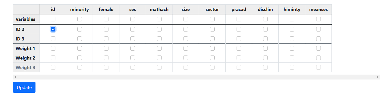
The first step is to indicate the ID variable, in this case
simply named ID.
 As there is no level-3 ID or weight variables in the current
example, the variables of interest are selected next.
As there is no level-3 ID or weight variables in the current
example, the variables of interest are selected next.
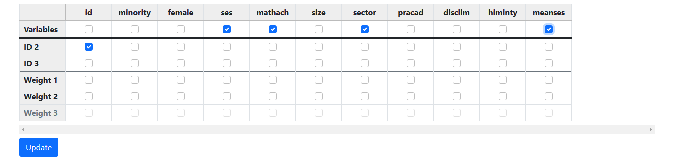 Clicking the Update button prompts the program to
check the data and perform an automatic assignment of variables to the
appropriate (student or school) levels.
Clicking the Update button prompts the program to
check the data and perform an automatic assignment of variables to the
appropriate (student or school) levels.
 The variable SECTOR and MEANSES are correctly indicated as
school level variables, while the outcome of interest here, MATHACH, and the
individual student SES are indicated as student level variables.
Having completed the Data File Specification, we are
ready to start building the model. To do so, we move on to the Models
page by clicking on the Models link at the top of the window.
Note that if data file specification is not completed, the Models
page will simply display the message
The variable SECTOR and MEANSES are correctly indicated as
school level variables, while the outcome of interest here, MATHACH, and the
individual student SES are indicated as student level variables.
Having completed the Data File Specification, we are
ready to start building the model. To do so, we move on to the Models
page by clicking on the Models link at the top of the window.
Note that if data file specification is not completed, the Models
page will simply display the message
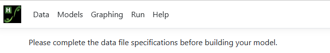 prompting the user to first complete the file specification
step. Model building only becomes possible once data file specification has
been completed.
prompting the user to first complete the file specification
step. Model building only becomes possible once data file specification has
been completed.
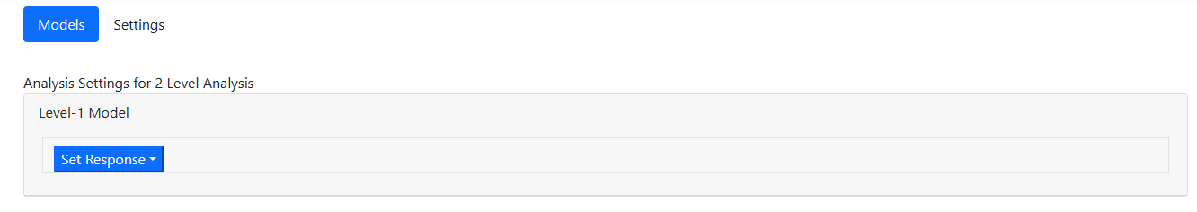
Model building
When the Models page is opened, the only active field
displayed is the Set Response option in the Level-1 Model field.
The program assumes the outcome variable of interest to be at the lowest level
of the hierarchy, and selecting this variable is the starting point for model
specification.
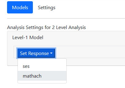
 In the current example, we are interested in the mathematical scores of
students, so we select the variable MATHACH from this drop-down list as shown
below
In the current example, we are interested in the mathematical scores of
students, so we select the variable MATHACH from this drop-down list as shown
below
 after which the program automatically updates the contents
of the Model page to display an unconditional two-level model with
MATHACH as outcome.
after which the program automatically updates the contents
of the Model page to display an unconditional two-level model with
MATHACH as outcome.
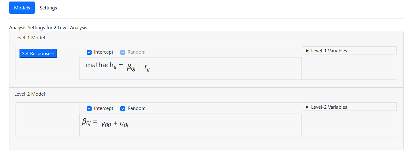 The Level-1 Variables and Level-2 Variables fields
are also activated in the process, so the next step is to start selecting
predictors from these lists.
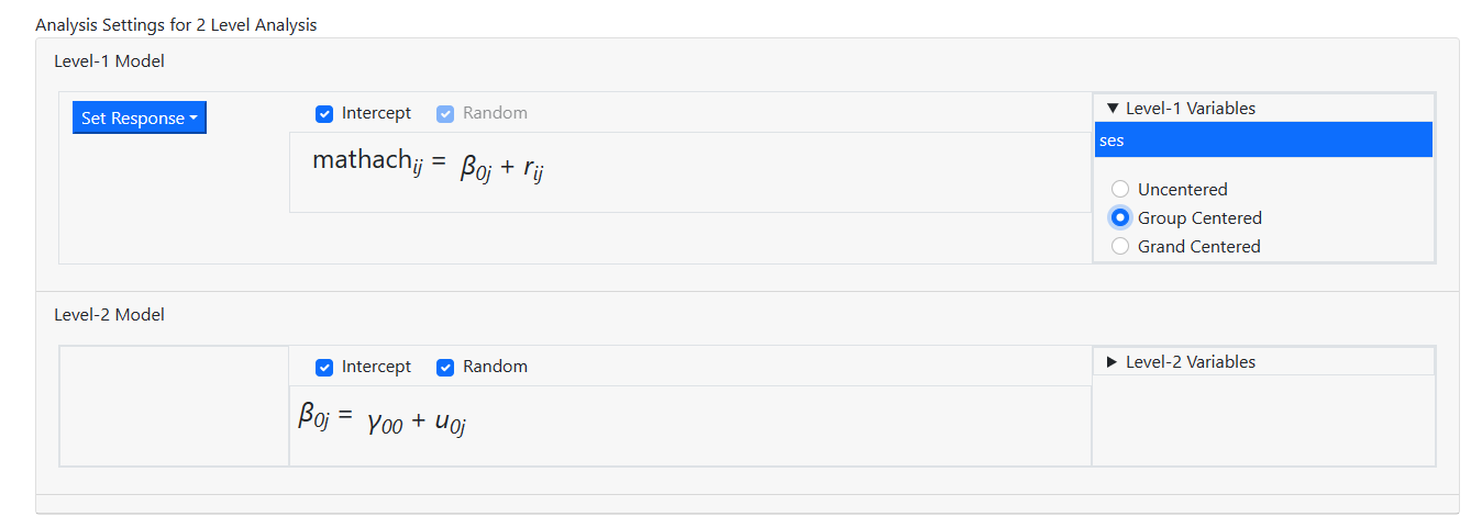
Recall from the discussion of the model previously that we
would like to include the level-1 predictor SES. Moreover, we would like to
include it as a group centered level-1 predictor. This is done by first
clicking on the variable name in the Level-1 Variables field and then
selecting the type of centering required. By default, it is assumed that
predictors are to be entered into the model uncentered. Here the radio button
for Group centered is checked to indicate that we want a group centered
predictor.
The Level-1 Variables and Level-2 Variables fields
are also activated in the process, so the next step is to start selecting
predictors from these lists.
Recall from the discussion of the model previously that we
would like to include the level-1 predictor SES. Moreover, we would like to
include it as a group centered level-1 predictor. This is done by first
clicking on the variable name in the Level-1 Variables field and then
selecting the type of centering required. By default, it is assumed that
predictors are to be entered into the model uncentered. Here the radio button
for Group centered is checked to indicate that we want a group centered
predictor.
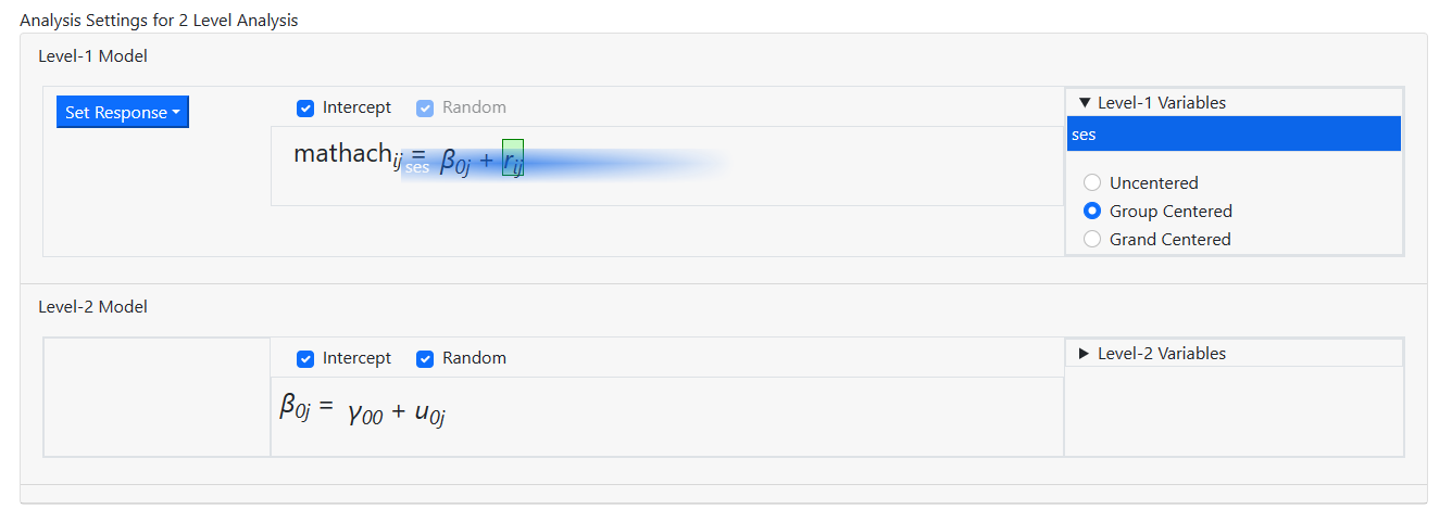
 Adding this variable to the level-1 equation is accomplished
by sampling dragging the variable name into the equation while holding the
mouse button down, releasing it only when the variable is in the equation
field.
Adding this variable to the level-1 equation is accomplished
by sampling dragging the variable name into the equation while holding the
mouse button down, releasing it only when the variable is in the equation
field.
 Once the mouse button is released, the model is updated to
the following random intercept model.
Once the mouse button is released, the model is updated to
the following random intercept model.
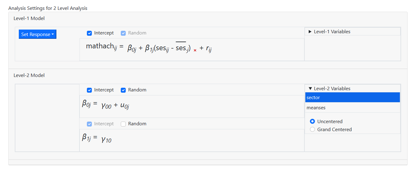
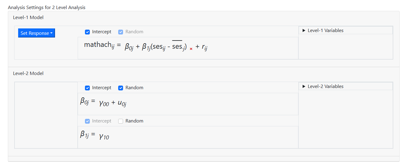 This completes the level-1 specification, and we can now add
the level-2 variables in a similar way using the Level-2 Variables
field. While it is possible to drag and drop multiple variables into the model
simultaneously, the current example calls for an uncentered and a grand mean
centered variable to both level-2 equations. As such, the two variables are
entered one by one. The first variable, SECTOR, is selected as
This completes the level-1 specification, and we can now add
the level-2 variables in a similar way using the Level-2 Variables
field. While it is possible to drag and drop multiple variables into the model
simultaneously, the current example calls for an uncentered and a grand mean
centered variable to both level-2 equations. As such, the two variables are
entered one by one. The first variable, SECTOR, is selected as
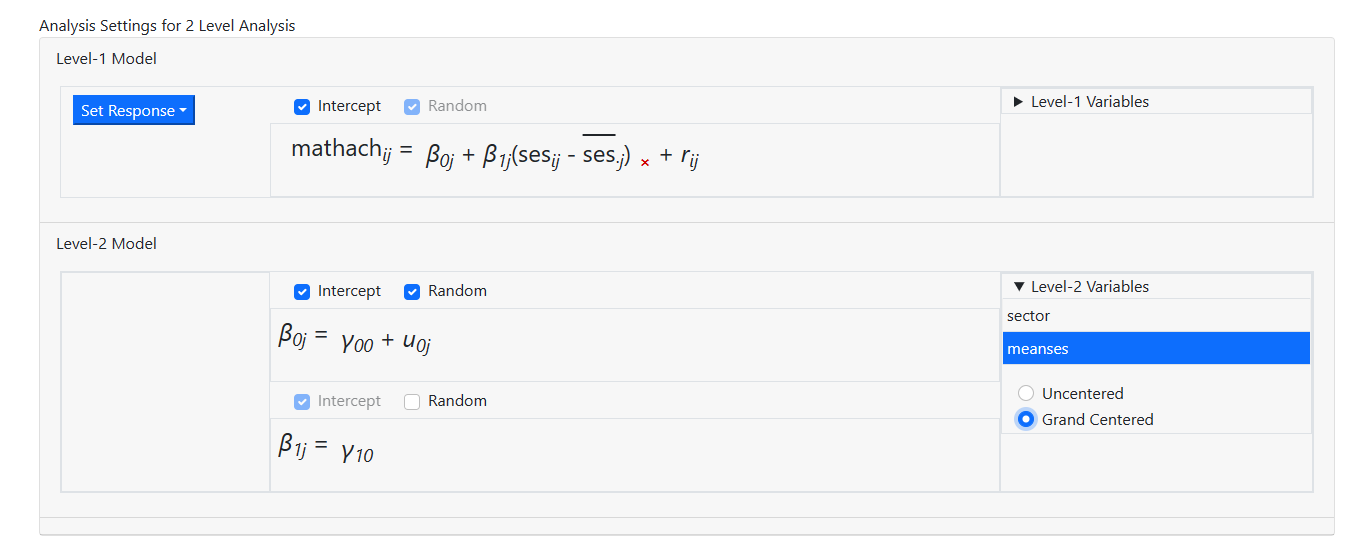
 while the grand mean centered MEANSES is entered as
 to obtain the model specification as shown below.
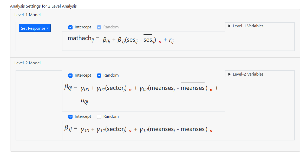 When this model is compared to that previously described, we
notice that we need to add a random slope for the level-1 predictor SES. To do
so, we simply click the Random check box above the slope equation. By
default, an intercept is always included in the higher-level equations. The
intercept may be removed, provided it is not the only effect on the equation of
interest.
The model is now complete
When this model is compared to that previously described, we
notice that we need to add a random slope for the level-1 predictor SES. To do
so, we simply click the Random check box above the slope equation. By
default, an intercept is always included in the higher-level equations. The
intercept may be removed, provided it is not the only effect on the equation of
interest.
The model is now complete
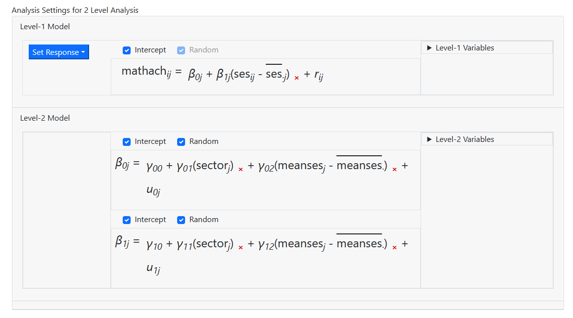 and we can move on to the Settings page to specify
the type of outcome.
and we can move on to the Settings page to specify
the type of outcome.
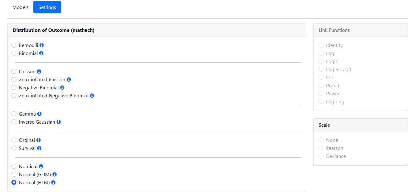
Specifying outcome type and other options
The Settings page is used to specify the type of
outcome used in the analysis. Additional options for the type of outcome can
also be selected on this page.
For the current model, we have a normally distributed continuous
outcome variable and we wish to fit a standard 2-level HLM model. The program
will automatically suggest the distribution type based on the data read in.
Ensure the option selected by the program is correct (see below). For a Normal
(HLM) model, no other options
are enabled on this page. As this page is complete, we click Save before
moving to the Run page, accessed by clicking the Run link at the
top of the window.
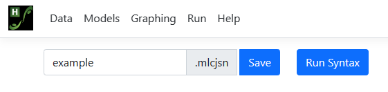
Running the model
The analysis is initiated via the Run page, accessed
via the Run link at the top of the window. The description of the data
and all options specified on the previous pages are captured in a JSON syntax
(file extension MLCJSN) that can be saved to a file with MLCJSN extension that
can be read back into the program, perhaps to serve a departure point for a
subsequent model.
To start the analysis, click the Run Syntax button.
 A Progress window will appear, giving details on the
iterative procedure. Links to all output files will
automatically appear on the Run page. Here we shows some of the HTML output at convergence. Note that a text version of the
output is also produced, containing the same information.
A Progress window will appear, giving details on the
iterative procedure. Links to all output files will
automatically appear on the Run page. Here we shows some of the HTML output at convergence. Note that a text version of the
output is also produced, containing the same information.
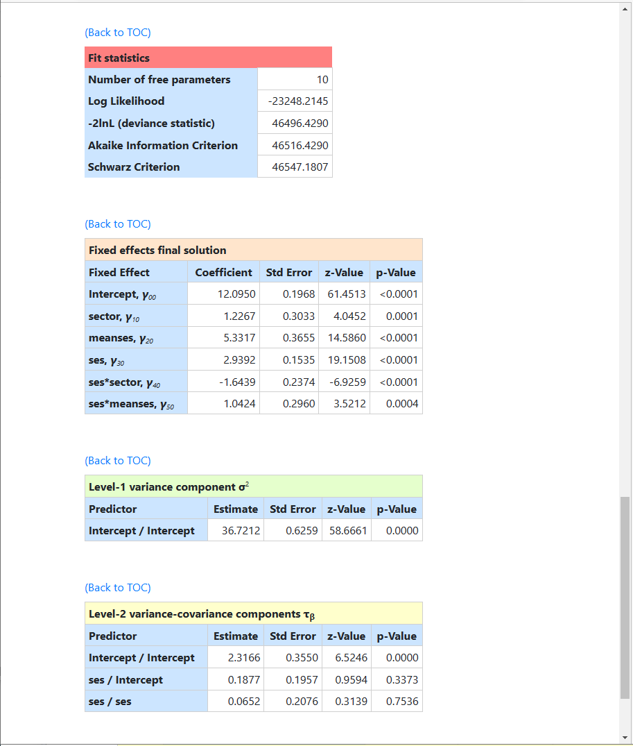 While all fixed effects are highly significant, the table of
Level-2 variance-covariance components shows that there is little evidence on a
significant SES slope.
While all fixed effects are highly significant, the table of
Level-2 variance-covariance components shows that there is little evidence on a
significant SES slope.